Synthetic Environments Data Tools and Visualization
We provide different functions and code snippets in Python to load Aria Synthetic Environments (ASE) data from a sequence and associate/interpret them with each other. The contents of each scene/sequence are detailed in Data Format.
They provide a set of helper functions to use the data efficiently and also visualize them. All of these snippets are placed under projectaria_tools/tree/main/projects/AriaSyntheticEnvironment/tutorial/code_snippets/
Data Helper Tools
These helper functions are broadly categorized into the following types:
- Data interpreter:
interpreter.py- Provides an interpreter for the ASE Scene Language to convert them into a 3D model in the form of bounding boxes
- Data readers:
readers.py- Provide readers for the:
ASE Scene LanguageGround-truth trajectorySemi-dense Map points
- Provide readers for the:
- Data Plotters:
plotters.py- Provide simple plotting functions for the:
3D scene from ASE Scene LanguageGround-truth trajectorySemi Dense Map points
- Provide simple plotting functions for the:
Visualization
Python sample
Viewer_projects_ase displays an interactive view of an ASE sequence with Rerun. It allows you to see all data in 3D context.
You can call as the following (frame_id being optional):
viewer_projects_ase --dataset_path ase_data/7 --frame_id 745
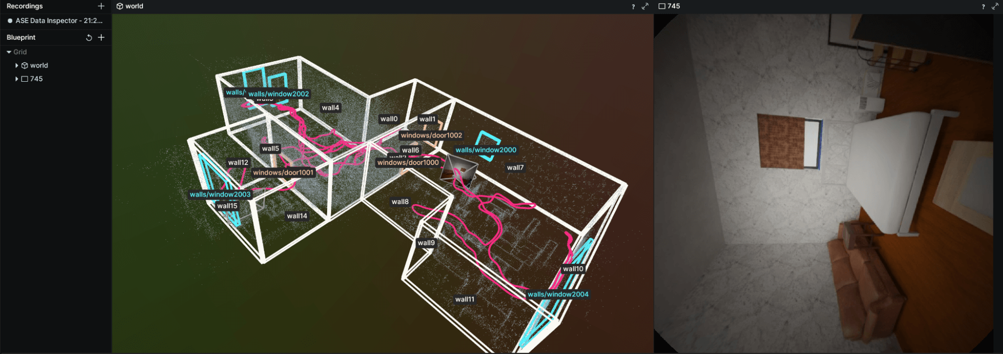
- The timeline enables you to switch before device_time and frame_id to know to which image frame_id a camera pose corresponds to
- The 3D world view is clickable, you can quickly select an object and see its instance name
Python Notebook
We also provide Jupyter notebooks to visualize the data for each sequence. To get started download ASE data following steps from Dataset Download
cd /path_to/projectaria_tools

jupyter notebook projects/AriaSyntheticEnvironment/tutorial/ase_tutorial_notebook.ipynb
Part 1: 3D visualization of the scene
This section will introduce the dataset’s 3D components as well as code snippets to help users get familiar with them.
You will be taken through examples of how to load the 3D dataset annotations namely: the ground-truth trajectory, the ASE Scene Language, and the Semi-dense Map point cloud. In addition, we provide examples of how they can each be plotted.
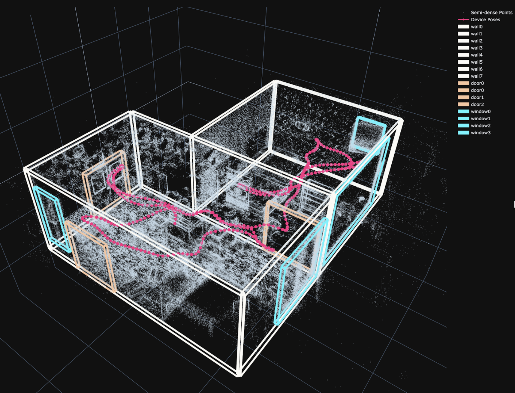
At the end of the section you should see 3D plots containing:
- The Semi-dense Map point cloud,
- The layout annotations, visualized as 3D box wireframes,
- The trajectory plotted as a dotted line in 3D.
Example scene visualization:
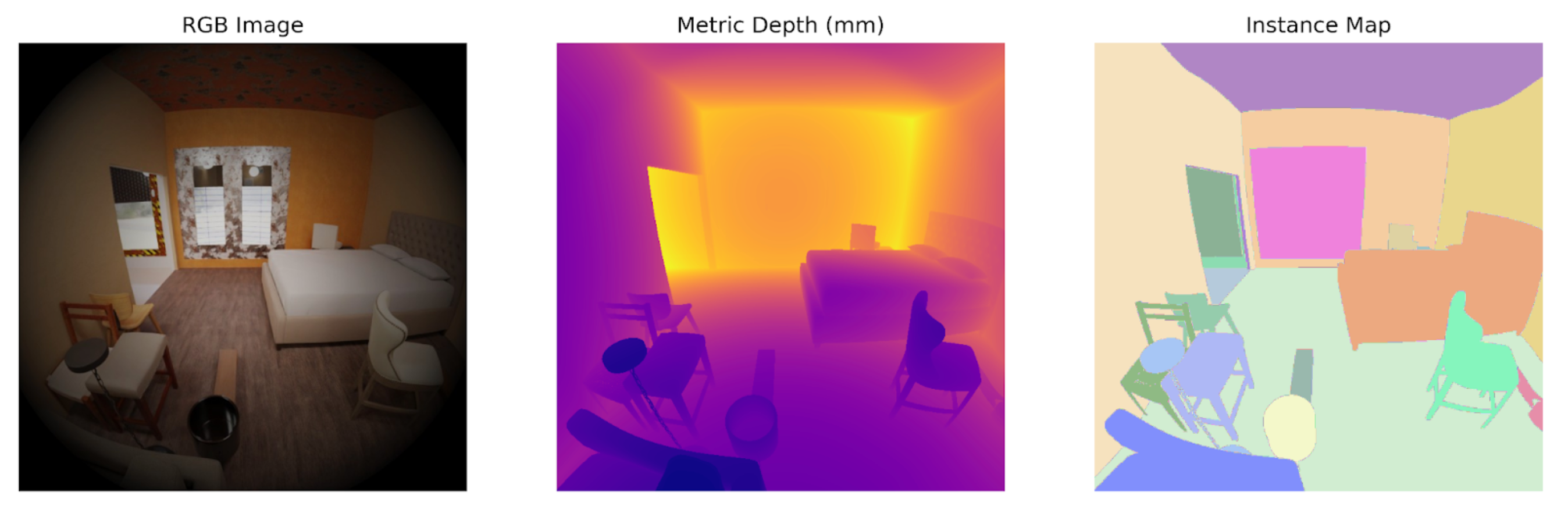
Part 2: Loading and Plotting Images and Image Annotations
Since the file structure and format are straightforward, the code consists of very simple PIL and matplotlib code to show the 3 images (RGB, depth and instance maps) side-by-side:
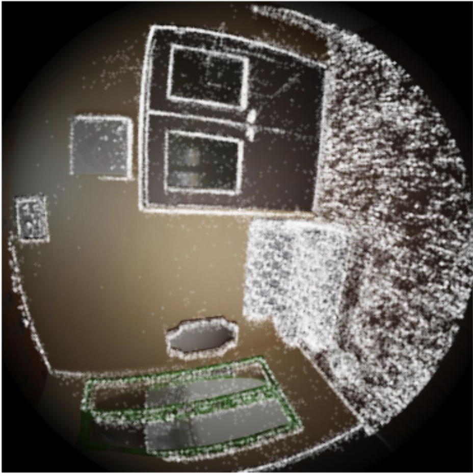
Part 3: Projecting Points into Images
Running the final part of the notebook will load the camera calibration, as well as the pointcloud, trajectory and select a random frame. Then given the device pose from the trajectory, we project the points into the frame.
Points that project outside of the valid radius, should not be plotted