IMU Noise Model for Project Aria Data

In our visual-inertial fusion algorithm, we model, as traditionally done, the stochastic part of the IMU error as including three components:

• Turn-on bias
• Bias random walk
• White noise

The noise along any of the axis of the inertial sensor is described as the sum of those contributions:

$$x^{\text{sampled}}_k = x^{\text{true}}_k + n^{\text{turn-on bias}}_{k0} + n^{\text{bias random walk}}_k + n^{\text{white noise}}_k$$

Where:

• $x^{\text{true}}_k$ is the real value of the quantity measured projected on the sensor sensitive axis.
• $x^{\text{sampled}}_k$ is the sampled value seen as a random variable.
• $n^{\text{turn-on bias}}_{k0}$ is a random variable draw from a Gaussian when the device is turned-on (denoted here as step $k_0$).
• $n^{\text{white noise}}_{k}$ is the time-independent noise components and draw from a 0-centered Gaussian at each step $k$.
  • The covariance of the Gaussian is usually characterized by the continuous noise $\sigma_c$ strength, which needs to be multiplied by the bandwidth (BW)h in Hz to get the distribution of the sample noise: $\sigma^2_c \cdot BW$.
  • $\sigma_c$ is sometimes called Angle Random walk in $rad/s/\sqrt{Hz}$ or $rad/\sqrt{s}$ for the gyrometer and the Velocity Random Walk in $m/s^2/\sqrt{Hz}$ or $m/s/\sqrt(s)$ for the accelerometer.
• $n^{\text{bias random walk}}_k$ is drawn from a random walk process.

The parameters describing those noises can be derived from an Allan Variance plot computed from data collected over a period of 24 hours in a temperature stable environment.

Table 1: White noise and bias instability parameters of Aria IMU sensors (1 gee = 9.81m/s^2)

	accel-left	accel-right	gyro-left	gyro-right
white noise ($\sigma_c$)	$0.9\times 10^{-4}\ \text{gees}/\sqrt{Hz}$	$0.8\times 10^{-4}\ \text{gees}/\sqrt{Hz}$	$5\times 10^{-3}\ \text{dps}/\sqrt{Hz}$	$1\times10^{-2}\ \text{dps}/\sqrt{Hz}$
bias instability	$2.8\times 10^{-5}\ \text{gees}$	$3.5\times 10^{-5}\ \text{gees}$	$1\times 10^{-3}\ \text{dps}$	$1.3\times10^{-3}\ \text{dps}$

The figure below shows the Allan Variance plot supporting this measurement.

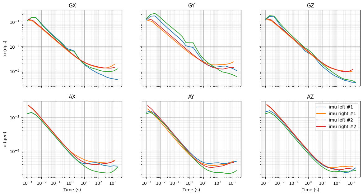Figure 1: Allan Variance plot computed from data collected over 24 hours in a temperature stable environment

With our sensor configuration for bandwidth, this leads to the following values for the sample noise:

Table 2: Sample noise of Aria IMU sensors

	accel-left (BW: 343Hz)	accel-right (BW: 353Hz)	gyro-left (BW:300Hz)	gyro-right (BW:116Hz)
$\sigma^{\text{white noise}}_k$	$16\times 10^{-3}\ m/s^2$	$15\times 10^{-3}\ m/s^2$	$1.5\times10^{-3}\ \text{rad/s}$	$1.8\times10^{-3}\ \text{rad/s}$

The data duration used for Allan Variance was not enough to capture the bias random walk confidently. This is because real MEMS sensors are not that well modelled by this stochastic model. To address this, we tune the parameter of the bias random walk used for sensor-fusion. We start from the bias instability measured on the Allan Variance of the sensor (the floor of the curve) and inflate it by a tuning factor.