Camera Intrinsic Models for Project Aria devices

This page provides an overview of the intrinsic models used by RGB, Eye Tracking and Mono Scene (aka SLAM) cameras in Project Aria glasses. Go to the Project Aria FAQ for more calibration information and resources.

A camera intrinsic model maps between a 3D world point in the camera coordinate and its corresponding 2D pixel on the sensor. It supports mapping from the 3D point to the pixel (projection) and from the pixel to the ray connecting the point and the camera's optical center.

Our projection models are based on polar coordinates of 3D world points. Given a 3D world point in the device frame $\mathbf{P}_d$, we first transform it to the camera's local frame

$$\mathbf{P}_c = (x, y, z) = T_\text{device}^\text{camera}\mathbf{P}_d$$

the corresponding polar coordinates $\Phi = (\theta, \varphi)$ that satisfies

$$x/z = \tan(\theta)\cos(\varphi), \quad y/z = \tan(\theta)\sin(\varphi).$$

We assume the camera has a single optical center and thus all points of the same polar coordinate maps to the same 2D pixel $\mathbf{p}$:

$$\mathbf{p} = f(\phi)$$

Here $f$ is the camera projection model.

Inversely, we can unproject from a 2D camera pixel to the polar coordinate by

$$\Phi = f^{-1}(\mathbf{p})$$

In Aria we support four types of project models, Linear, Spherical, KannalaBrandtK3, and FisheyeRadTanThinPrism. The linear camera model are standard textbook intrinsic models and good for image rectification. However, cameras on the Aria glasses all have fisheye lenses, and spherical camera model are much better approximations for these glasses. In order to calibrate the camera lenses at a high quality, we use two more sophisticated camera models to add modeling of radial and tangential distortions.

The next table shows which model is used for each type of Aria camera:

Camera Type	Intrinsics Model
Slam Camera	FisheyeRadTanThinPrism
Rgb Camera	FisheyeRadTanThinPrism
Eye-Tracking Camera	KannalaBrandtK3

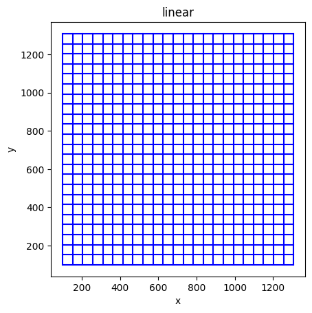
The linear camera model

The linear camera model (a.k.a pinhole model) is parametrized by 4 coefficients : f_x, f_y, c_x, c_y.

$(f_x, f_y)$ are the focal lengths, and $c_x, c_y$ are the coordinate of the projection of the optical axis. It maps from world point $(x,y,z)$ to 2D camera pixel $\mathbf{p}=(u, v)$ with the following formulae.

$$u = f_x x/z + c_x \\ v = f_y y/z + c_y$$

Or, in polar coordinates:

$$u = f_x tan(\theta) \cos(\varphi) + c_x, \\ v = f_y tan(\theta) \sin(\varphi) + c_y.$$

Inversely, we can unproject from 2D camera pixel $\mathbf{p}=(u, v)$ to the homogeneous coordinate of the world point by

$$x/z=(u-c_x)/f_x, \\ y/z=(v-c_y)/f_y.$$

The linear camera model preserves linearity in 3D space, thus straight lines in the real world are supposed to look straight under the linear camera model.

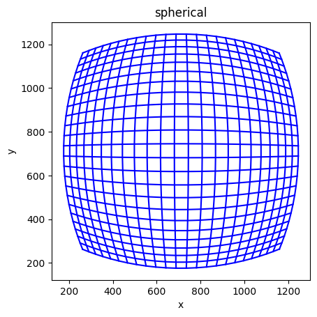
The spherical camera model

The spherical camera model is, similarly from the linear camera model parametrized by 4 coefficients : f_x, f_y, c_x, c_y. The pixel coordinates are linear to solid angles rather than the homography coordinate system. The projection function can be written in polar coordinates

$$u = f_x \theta \cos(\varphi) + c_x, \\ v = f_y \theta \sin(\varphi) + c_y.$$

Note the difference from the linear camera model — under spherical projection, 3D straight lines look curved in images.

Inversely, we can unproject from 2D camera pixel $\mathbf{p}=(u, v)$ to the homogeneous coordinate of the world point by

$$\theta = \sqrt{(u - c_x)^2/f_x^2 + (v - c_y)^2/f_y^2}, \\ \varphi = \arctan((u - c_x)/f_x, (v - c_y)/f_y).$$

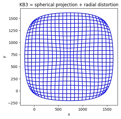
The KannalaBrandtK3 (KB3) model

The KannalaBrandtK3 model adds radial distortion to the linear model

$$u = f_x r(\theta) \cos(\varphi) + c_x, \quad v = f_y r(\theta) \sin(\varphi) + c_y.$$

where

$$r(\theta) = \theta + k_0 \theta^3 + k_1 \theta^5 + k_2 \theta^7 + k_3 \theta^9 + ...$$

In KannalaBrandtK3 model we use a 9-th order polynomial with four radial distortion parameters $k_0, ... k_3$.

To unproject from camera pixel $(u, v)$ to the world point $(\theta, \varphi)$, we first compute

$$\varphi = \arctan((u - c_x)/f_x, (v - c_y)/f_y) \\ r(\theta) = \sqrt{(u - c_x)^2/f_x^2 + (v - c_y)^2/f_y^2}$$

Then we use Newton method to inverse the function $r(\theta)$ to compute $\theta$. See the code here.

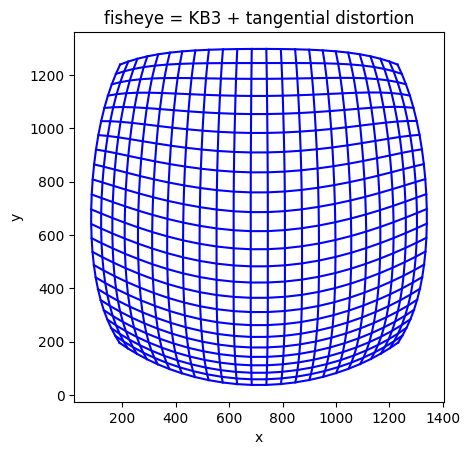
The Fisheye62 model

The Fisheye62 model adds tangential distortion on top of the KB3 model parametrized by two new coefficients: p_0 p_1.

$$u = f_x . (u_r + t_x(u_r, v_r)) + c_x, \\ v = f_y . (v_r + t_y(u_r, v_r)) + c_y.$$

where

$$u_r = r(\theta) \cos(\varphi), \\ v_r = r(\theta) \sin(\varphi).$$

and

$$t_x(u_r, v_r) = p_0(2 u_r^2 + r(\theta)^2) + 2p_1u_rv_r, \\ t_y(u_r, v_r) = p_1(2 v_r^2 + r(\theta)^2) + 2p_0u_rv_r.$$

To unproject from camera pixel $(u, v)$ to the world point $(\theta, \varphi)$, we first use Newton method to compute $u_r$ and $v_r$ from $(u - c_x)/f_x$ and $(v - cy)/f_y$, and then compute $(\theta, \varphi)$ using the above KB3 unproject method.

The FisheyeRadTanThinPrism (Fisheye624) model

The FisheyeRadTanThinPrism (also called Fisheye624 in file and codebase) models thin-prism distortion (noted $tp$) on top of the Fisheye62 model above. Its parametrization contains 4 additional coefficients: s_0 s_1 s_2 s_3. The projection function writes:

$$u = f_x \cdot (u_r + t_x(u_r, v_r) + tp_x(u_r, v_r)) + c_x, \\ v = f_y \cdot (v_r + t_y(u_r, v_r) + tp_y(u_r, v_r)) + c_y.$$

u_r, v_r, t_x, t_y are defined as in the Fisheye62 model, while $tp_x$ and $tp_y$ are defined as:

$$tp_x(u_r, v_r) = s_0 r(\theta)^2 + s_1 r(\theta)^4, \\ tp_y(u_r, v_r) = s_2 r(\theta)^2 + s_3 r(\theta)^4.$$

To unproject from camera pixel $(u, v)$ to the world point $(\theta, \varphi)$, we first use Newton method to compute $u_r$ and $v_r$ from $(u - c_x)/f_x$ and $(v - cy)/f_y$, and then compute $(\theta, \varphi)$ using the above KB3 unproject method.

Note that in practice, in our codebase and calibration file we assume $f_x$ and $f_y$ are equal.