Metrics across Ranks
“A chain is only as strong as its weakest link.” A similar analogy applies in performance computing in distributed system. When training models with multiple GPUs and machines, if one rank is (significantly) slower than the rest, the whole system operates at the speed of the slow one.
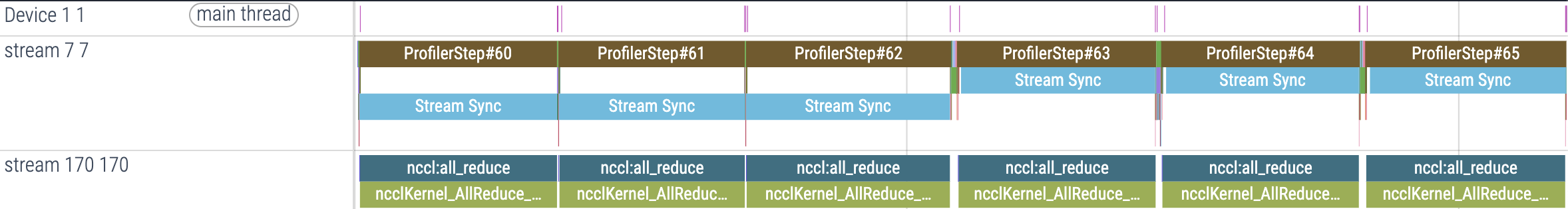
When this happens, the faster ranks wait for the slow rank for the
communication. If you trace the pipeline with
PyTorch Profiler,
you can see them blocked typically at nccl:all_reduce as follow.
(and when this happens, the SM utilization of GPU does not go above around 20%.)
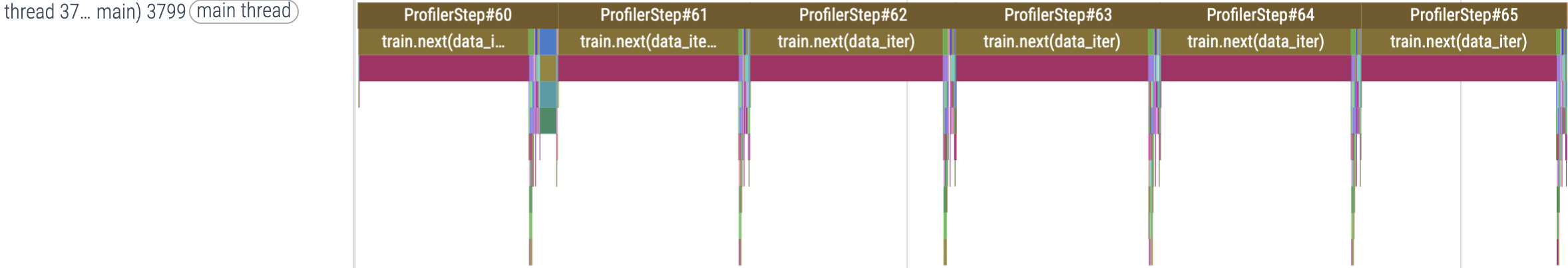
And if the bottleneck of the slow rank is data loading (which is almost always
the case), then the trace of the rank shows that it is blocked on
next(dataloader).
There are many possibilities this can happen. SPDL’s performance statistics can help identify the cause.
Data Readiness
We had a case where the data loading is slow for a particular rank. The following plot shows the data readiness at sink queue for all the ranks.
The rank 0 and 19 clearly shows different trands than the rest. When a rank becomes significantly slower than the rest, the other ranks have spare time waiting for the slow one. This allows the data loading pipeline to do more work, and fill the buffer queue. Therefore the data readiness of the other ranks can stay near 1, while the data readiness of the slowest node stays 0, because the data is immediately consumed.
Now let’s try to locate the bottleneck. This pipeline is composed of download, decompress and (batch) preprocessing as illustrated follow.
The following plots show the data readiness for the stage preceding the sink.
The data readiness of the decompress stage is always almost 1 across the ranks, while the data readiness of the preprocess stage somewhat resembles that of the sink queue.
These observations suggest that the bottleneck is in the preprocess stage. So the next action we should take is to figure out why preprocessing can be slower.
(For this particular case, the data is time series with different signal length, so we suspect that the time complexity of preprocessing is not constant but grows as the signal length become larger.)
Average Download Time
Another statistics worth checking across the ranks is the average time for downloading stage. The time for downloading data can be affected by many factors. The following is some common cases.
Disruption in the network.
The training node and the remote data storage are in different available zone.
The remote storage system applies throttling.
When such disruption happens, we can see it through the average time for download stage.
We take an example from a production pipeline consists of 3 machines, each of which is equipped with 8 GPUs. The following plot shows the average download time across the ranks.
Before 7 AM, the average download time is around 2 -3 second. After 7 AM, all ranks experience increased downloading time with higher variance.
By checking the log on the storage system, we verified that this was caused by throttling. Past 8:30 AM, we can see that the node 2 (rank 16 to 23) is receiving a different level of throttling than node 0 (rank 0 to 7) and 1 (rank 8 to 15). The speed of the pipeline is governed by the throttling applied to the node 2.