This 1–2 hour tutorial is intended for classrooms, workshops, and guided self-study. It combines several UMA workflows in one linear lesson. The same topics also appear as shorter, task-focused pages elsewhere in the documentation; use Hello World if you only need a concise introduction.
This tutorial walks through representative ways to use UMA. It is best suited to researchers who are new to UMA and already have some familiarity with ASE and molecular simulation.
Before you start / installation
You need to get a HuggingFace account and request access to the UMA models.
You need a Huggingface account, request access to https://
Permissions: Read access to contents of all public gated repos you can access
Then, add the token as an environment variable (using huggingface-cli login:
# Enter token via huggingface-cli
! huggingface-cli login
or you can set the token via HF_TOKEN variable:
# Set token via env variable
import os
os.environ['HF_TOKEN'] = 'MYTOKEN'
Installation process
It may be enough to use pip install fairchem-core. This gets you the latest version on PyPi (https://
Here we install some sub-packages. This can take 2-5 minutes to run.
! pip install fairchem-core fairchem-data-oc fairchem-applications-cattsunami x3dase# Check that packages are installed
!pip list | grep fairchemfairchem-applications-cattsunami 1.1.2.dev403+g3801dac0c
fairchem-core 2.23.1.dev4+g3801dac0c
fairchem-data-oc 1.0.3.dev403+g3801dac0c
fairchem-data-omat 0.2.1.dev308+g3801dac0c
import fairchem.core

fairchem.core.__version__
Warp 1.18.0 initialized:
CUDA Toolkit 13.4, Driver 13.1
Devices:
"cpu" : "x86_64"
"cuda:0" : "Tesla T4" (16 GiB, sm_75, mempool enabled)
Kernel cache:
/home/runner/.cache/warp/1.18.0
'2.23.1.dev4+g3801dac0c'Illustrative examples
These should just run, and are here to show some basic uses.
Spin gap energy - OMOL
This is the difference in energy between a triplet and single ground state for a CH2 radical. This downloads a ~1GB checkpoint the first time you run it.
We don’t set a device here, so we get a warning about using a CPU device. You can ignore that. If a CUDA environment is available, a GPU may be used to speed up the calculations.
from fairchem.core import FAIRChemCalculator, pretrained_mlip

predictor = pretrained_mlip.get_predict_unit("uma-s-1p2p1")
WARNING:root:device was not explicitly set, using device='cuda'.
from ase.build import molecule

#  singlet CH2
singlet = molecule("CH2_s1A1d")
singlet.info.update({"spin": 1, "charge": 0})
singlet.calc = FAIRChemCalculator(predictor, task_name="omol")

#  triplet CH2
triplet = molecule("CH2_s3B1d")
triplet.info.update({"spin": 3, "charge": 0})
triplet.calc = FAIRChemCalculator(predictor, task_name="omol")

print(triplet.get_potential_energy() - singlet.get_potential_energy())
WARNING:root:Model is being compiled this might take a while for the first time
W1007 03:04:22.565000 9826 site-packages/torch/_logging/_internal.py:1345] [0/0] Profiler record function <class 'torch.autograd.profiler.record_function'> will be ignored
WARNING:root:The UMA fast path (merge_mole + compile) is only available for fixed composition, task, charge, and spin. This is optimized for MD applications. Falling back to a less optimized version for subsequent evaluations. Reason: 'Spin differs: tensor([3]) vs tensor([1], device='cuda:0')'.
Use inference_settings='batch' for heterogeneous batched evaluations.
-0.3581800059773741
Example of adsorbate relaxation - OC20
Here we just setup a Cu(100) slab with a CO on it and relax it.
We specify an explicit device in the predictor here, and avoid the warning.
from ase.build import add_adsorbate, fcc100, molecule
from ase.optimize import LBFGS
from fairchem.core import FAIRChemCalculator, pretrained_mlip

predictor = pretrained_mlip.get_predict_unit("uma-s-1p2p1")
calc = FAIRChemCalculator(predictor, task_name="oc20")

# Set up your system as an ASE atoms object
slab = fcc100("Cu", (3, 3, 3), vacuum=8, periodic=True)

adsorbate = molecule("CO")
add_adsorbate(slab, adsorbate, 2.0, "bridge")
slab.calc = calc

# Set up LBFGS dynamics object
opt = LBFGS(slab)
opt.run(0.05, 100)
print(slab.get_potential_energy())
WARNING:root:device was not explicitly set, using device='cuda'.
WARNING:root:Model is being compiled this might take a while for the first time
W1007 03:06:17.640000 9826 site-packages/torch/_inductor/utils.py:1953] [6/1] Not enough SMs to use max_autotune_gemm mode
/home/runner/work/_tool/Python/3.12.15/x64/lib/python3.12/site-packages/torch/_inductor/lowering.py:2352: FutureWarning: `torch._prims_common.check` is deprecated and will be removed in the future. Please use `torch._check*` functions instead.
  check(
       Step     Time          Energy          fmax
LBFGS:    0 03:07:21      -89.681337       11.323903
LBFGS:    1 03:07:21      -92.566008        6.206132
LBFGS:    2 03:07:21      -92.725428        7.225987
LBFGS:    3 03:07:21      -93.076594        3.480319
LBFGS:    4 03:07:21      -93.232398        3.197181
LBFGS:    5 03:07:21      -93.337015        2.257560
LBFGS:    6 03:07:21      -93.578594        1.131644
LBFGS:    7 03:07:21      -93.667721        0.962640
LBFGS:    8 03:07:21      -93.776322        0.594680
LBFGS:    9 03:07:22      -93.855048        0.453787
LBFGS:   10 03:07:22      -93.890289        0.343756
LBFGS:   11 03:07:22      -93.907597        0.323595
LBFGS:   12 03:07:22      -93.933876        0.534155
LBFGS:   13 03:07:22      -93.946599        0.364662
LBFGS:   14 03:07:22      -93.953996        0.148299
LBFGS:   15 03:07:22      -93.958750        0.167811
LBFGS:   16 03:07:22      -93.965452        0.254314
LBFGS:   17 03:07:22      -93.971903        0.264227
LBFGS:   18 03:07:22      -93.976651        0.149766
LBFGS:   19 03:07:23      -93.978217        0.045404
-93.97821687397828
Example bulk relaxation - OMAT
from ase.build import bulk
from ase.filters import FrechetCellFilter
from ase.optimize import FIRE
from fairchem.core import FAIRChemCalculator, pretrained_mlip

predictor = pretrained_mlip.get_predict_unit("uma-s-1p2p1")
calc = FAIRChemCalculator(predictor, task_name="omat")

atoms = bulk("Fe")
atoms.calc = calc

opt = FIRE(FrechetCellFilter(atoms))
opt.run(0.05, 100)

print(atoms.get_stress())  # !!!! We get stress now!
WARNING:root:device was not explicitly set, using device='cuda'.
WARNING:root:Model is being compiled this might take a while for the first time
      Step     Time          Energy          fmax
FIRE:    0 03:08:59       -8.261835        0.581869
FIRE: 1 03:08:59 -8.268777 0.204166
FIRE: 2 03:09:00 -8.266207 0.459185
FIRE:    3 03:09:00       -8.267596        0.348396
FIRE:    4 03:09:00       -8.269143        0.164887
FIRE:    5 03:09:01       -8.269600        0.035843
[ 3.10668046e-03  3.10667916e-03  3.10679920e-03 -1.29563281e-08
 -4.24853225e-09  9.78575027e-09]
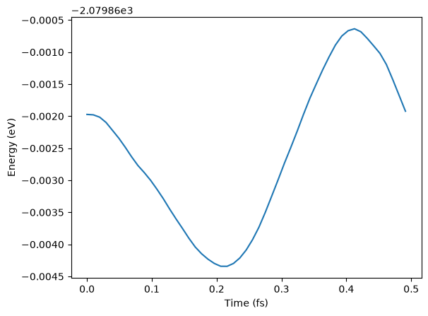
Molecular dynamics - OMOL
import matplotlib.pyplot as plt

from ase import units
from ase.build import molecule
from ase.io import Trajectory
from ase.md.langevin import Langevin
from fairchem.core import FAIRChemCalculator, pretrained_mlip

predictor = pretrained_mlip.get_predict_unit("uma-s-1p2p1")
calc = FAIRChemCalculator(predictor, task_name="omol")

atoms = molecule("H2O")
atoms.info.update(charge=0, spin=1)  # For omol

atoms.calc = calc

dyn = Langevin(
    atoms,
    timestep=0.1 * units.fs,
    temperature_K=400,
    friction=0.001 / units.fs,
)

trajectory = Trajectory("my_md.traj", "w", atoms)
dyn.attach(trajectory.write, interval=1)
dyn.run(steps=50)

# See some results - not paper ready!
traj = Trajectory("my_md.traj")
plt.plot(
    [i * 0.1 * units.fs for i in range(len(traj))],
    [a.get_potential_energy() for a in traj],
)
plt.xlabel("Time (fs)")
plt.ylabel("Energy (eV)");
WARNING:root:device was not explicitly set, using device='cuda'.
/home/runner/work/_tool/Python/3.12.15/x64/lib/python3.12/site-packages/ase/md/langevin.py:102: FutureWarning: The implementation of `fixcm=True` in `Langevin` does not strictly sample the correct NVT distributions. The deviations are typically small for large systems but can be more pronounced for small systems. Use `fixcm=False` together with `ase.constraints.FixCom`. `fixcm` is deprecated since ASE 3.28.0 and will be removed in a future release.
  warnings.warn(msg, FutureWarning)
WARNING:root:Model is being compiled this might take a while for the first time
Catalyst Adsorption energies
The basic approach in computing an adsorption energy is to compute this energy difference:
dH = E_adslab - E_slab - E_adsWe use UMA for two of these energies E_adslab and E_slab. For E_ads We have to do something a little different. The OC20 task is not trained for molecules or molecular fragments. We use atomic energy reference energies instead. These are tabulated below.
The OC20 reference scheme is this reaction:
x CO + (x + y/2 - z) H2 + (z-x) H2O + w/2 N2 + * -> CxHyOzNw*For this example we have
-H2 + H2O + * -> O*. "O": -7.204 eVWhere "O": -7.204 is a constant.
To get the desired reaction energy we want we add the formation energy of water. We use either DFT or experimental values for this reaction energy.
1/2O2 + H2 -> H2OAlternatives to this approach are using DFT to estimate the energy of 1/2 O2, just make sure to use consistent settings with your task. You should not use OMOL for this.
from ase.build import add_adsorbate, fcc111
from ase.optimize import BFGS
from fairchem.core import FAIRChemCalculator, pretrained_mlip

predictor = pretrained_mlip.get_predict_unit("uma-s-1p2p1")
calc = FAIRChemCalculator(predictor, task_name="oc20")
WARNING:root:device was not explicitly set, using device='cuda'.
# reference energies from a linear combination of H2O/N2/CO/H2!
atomic_reference_energies = {
    "H": -3.477,
    "N": -8.083,
    "O": -7.204,
    "C": -7.282,
}

re1 = -3.03  # Water formation energy from experiment

slab = fcc111("Pt", size=(2, 2, 5), vacuum=20.0)
slab.pbc = True

adslab = slab.copy()
add_adsorbate(adslab, "O", height=1.2, position="fcc")

slab.calc = calc
opt = BFGS(slab)
print("Relaxing slab")
opt.run(fmax=0.05, steps=100)
slab_e = slab.get_potential_energy()

adslab.calc = calc
opt = BFGS(adslab)
print("\nRelaxing adslab")
opt.run(fmax=0.05, steps=100)
adslab_e = adslab.get_potential_energy()
Relaxing slab
WARNING:root:Model is being compiled this might take a while for the first time
      Step     Time          Energy          fmax
BFGS:    0 03:09:21     -104.713230        0.695698
BFGS:    1 03:09:21     -104.770832        0.592989
BFGS:    2 03:09:21     -104.910088        0.340089
BFGS:    3 03:09:21     -104.937704        0.411474
BFGS:    4 03:09:21     -105.009222        0.454688
BFGS:    5 03:09:21     -105.068384        0.352782
WARNING:root:The UMA fast path (merge_mole + compile) is only available for fixed composition, task, charge, and spin. This is optimized for MD applications. Falling back to a less optimized version for subsequent evaluations. Reason: 'Compositions differ from merged model'.
Use inference_settings='batch' for heterogeneous batched evaluations.
BFGS:    6 03:09:21     -105.105353        0.173401
BFGS:    7 03:09:21     -105.116032        0.042068

Relaxing adslab
      Step     Time          Energy          fmax
BFGS:    0 03:09:28     -110.098581        1.709169
BFGS:    1 03:09:28     -110.275966        0.961389
BFGS: 2 03:09:28 -110.420420 0.724063
BFGS: 3 03:09:29 -110.468240 0.788379
BFGS: 4 03:09:29 -110.569490 0.640718
BFGS: 5 03:09:29 -110.633821 0.473709
BFGS: 6 03:09:29 -110.685971 0.559150
BFGS: 7 03:09:30 -110.731265 0.612414
BFGS: 8 03:09:30 -110.762440 0.457343
BFGS: 9 03:09:30 -110.776664 0.240138
BFGS: 10 03:09:30 -110.780696 0.109518
BFGS: 11 03:09:30 -110.781686 0.093772
BFGS: 12 03:09:31 -110.782524 0.057410
BFGS: 13 03:09:31 -110.783130 0.043505
Now we compute the adsorption energy.
# Energy for ((H2O-H2) + * -> *O) + (H2 + 1/2O2 -> H2O) leads to 1/2O2 + * -> *O!
adslab_e - slab_e - atomic_reference_energies["O"] + re1-1.4930972654475805How did we do? We need a reference point. In the paper below, there is an atomic adsorption energy for O on Pt(111) of about -4.264 eV. This is for the reaction O + * -> O*. To convert this to the dissociative adsorption energy, we have to add the reaction:
1/2 O2 -> O D = 2.58 eV (expt)to get a comparable energy of about -1.68 eV. There is about ~0.2 eV difference (we predicted -1.47 eV above, and the reference comparison is -1.68 eV) to account for. The biggest difference is likely due to the differences in exchange-correlation functional. The reference data used the PBE functional, and eSCN was trained on RPBE data. To additional places where there are differences include:
Difference in lattice constant
The reference energy used for the experiment references. These can differ by up to 0.5 eV from comparable DFT calculations.
How many layers are relaxed in the calculation
Some of these differences tend to be systematic, and you can calibrate and correct these, especially if you can augment these with your own DFT calculations.
It is always a good idea to visualize the geometries to make sure they look reasonable.
import matplotlib.pyplot as plt
from ase.visualize.plot import plot_atoms

fig, axs = plt.subplots(1, 2)
plot_atoms(slab, axs[0])
plot_atoms(slab, axs[1], rotation=("-90x"))
axs[0].set_axis_off()
axs[1].set_axis_off()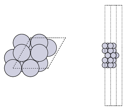
fig, axs = plt.subplots(1, 2)
plot_atoms(adslab, axs[0])
plot_atoms(adslab, axs[1], rotation=("-90x"))
axs[0].set_axis_off()
axs[1].set_axis_off()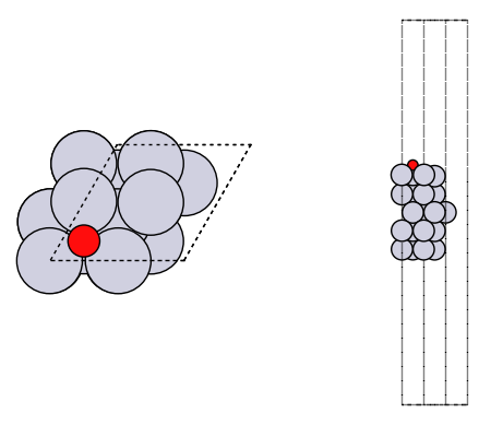
Molecular vibrations
from ase import Atoms
from ase.optimize import BFGS

predictor = pretrained_mlip.get_predict_unit("uma-s-1p2p1")
calc = FAIRChemCalculator(predictor, task_name="omol")

from ase.vibrations import Vibrations

n2 = Atoms("N2", [(0, 0, 0), (0, 0, 1.1)])
n2.info.update({"spin": 1, "charge": 0})
n2.calc = calc

BFGS(n2).run(fmax=0.01)
WARNING:root:device was not explicitly set, using device='cuda'.
WARNING:root:Model is being compiled this might take a while for the first time
      Step     Time          Energy          fmax
BFGS:    0 03:09:43    -2981.068400        1.649248
BFGS:    1 03:09:43    -2980.961396        6.657440
BFGS:    2 03:09:43    -2981.077198        0.215419
BFGS:    3 03:09:43    -2981.077343        0.027041
BFGS:    4 03:09:43    -2981.077344        0.000126
np.True_vib = Vibrations(n2)
vib.run()
vib.summary()---------------------
# meV cm^-1
---------------------
0 0.0i 0.0i
1 0.0i 0.0i
2 0.0i 0.0i
3 2.0 16.0
4 2.0 16.0
5 309.2 2493.7
---------------------
Zero-point energy: 0.157 eV
Bulk alloy phase behavior
Adapted from https://
We manually compute the formation energy of pure compounds and some alloy compositions to assess stability.
from ase.atoms import Atom, Atoms
from ase.filters import FrechetCellFilter
from ase.optimize import FIRE
from fairchem.core import FAIRChemCalculator, pretrained_mlip

predictor = pretrained_mlip.get_predict_unit("uma-s-1p2p1")

cu = Atoms(
    [Atom("Cu", [0.000, 0.000, 0.000])],
    cell=[[1.818, 0.000, 1.818], [1.818, 1.818, 0.000], [0.000, 1.818, 1.818]],
    pbc=True,
)
cu.calc = FAIRChemCalculator(predictor, task_name="omat")

opt = FIRE(FrechetCellFilter(cu))
opt.run(0.05, 100)

cu.get_potential_energy()
WARNING:root:device was not explicitly set, using device='cuda'.
WARNING:root:Model is being compiled this might take a while for the first time
      Step     Time          Energy          fmax
FIRE:    0 03:09:52       -3.747320        0.177137
FIRE:    1 03:09:52       -3.748121        0.124314
FIRE: 2 03:09:52 -3.748826 0.030733
-3.7488258397439216pd = Atoms(
[Atom("Pd", [0.000, 0.000, 0.000])],
cell=[[1.978, 0.000, 1.978], [1.978, 1.978, 0.000], [0.000, 1.978, 1.978]],
pbc=True,
)
pd.calc = FAIRChemCalculator(predictor, task_name="omat")
opt = FIRE(FrechetCellFilter(pd))
opt.run(0.05, 100)
pd.get_potential_energy()WARNING:root:The UMA fast path (merge_mole + compile) is only available for fixed composition, task, charge, and spin. This is optimized for MD applications. Falling back to a less optimized version for subsequent evaluations. Reason: 'Compositions differ from merged model'.
Use inference_settings='batch' for heterogeneous batched evaluations.
      Step     Time          Energy          fmax
FIRE:    0 03:10:00       -5.211659        0.162688
FIRE: 1 03:10:00 -5.212260 0.083200
FIRE: 2 03:10:00 -5.212418 0.040824
-5.212418248939699Alloy formation energies
cupd1 = Atoms(
    [Atom("Cu", [0.000, 0.000, 0.000]), Atom("Pd", [-1.652, 0.000, 2.039])],
    cell=[[0.000, -2.039, 2.039], [0.000, 2.039, 2.039], [-3.303, 0.000, 0.000]],
    pbc=True,
)  # Note pbc=True is important, it is not the default and OMAT

cupd1.calc = FAIRChemCalculator(predictor, task_name="omat")

opt = FIRE(FrechetCellFilter(cupd1))
opt.run(0.05, 100)

cupd1.get_potential_energy()
Step Time Energy fmax
FIRE: 0 03:10:01 -9.196722 0.119175
FIRE: 1 03:10:01 -9.196860 0.110741
FIRE: 2 03:10:02 -9.197097 0.095550
FIRE: 3 03:10:02 -9.197386 0.076958
FIRE: 4 03:10:03 -9.197713 0.059664
FIRE: 5 03:10:03 -9.198107 0.064212
FIRE: 6 03:10:04 -9.198606 0.066553
FIRE: 7 03:10:04 -9.199217 0.059752
FIRE: 8 03:10:04 -9.199986 0.066175
FIRE: 9 03:10:05 -9.200899 0.083518
FIRE: 10 03:10:05 -9.201996 0.093695
FIRE: 11 03:10:06 -9.203361 0.086995
FIRE: 12 03:10:06 -9.204967 0.062412
FIRE: 13 03:10:07 -9.206710 0.048801
-9.206710263668349cupd2 = Atoms(
[
Atom("Cu", [-0.049, 0.049, 0.049]),
Atom("Cu", [-11.170, 11.170, 11.170]),
Atom("Pd", [-7.415, 7.415, 7.415]),
Atom("Pd", [-3.804, 3.804, 3.804]),
],
cell=[[-5.629, 3.701, 5.629], [-3.701, 5.629, 5.629], [-5.629, 5.629, 3.701]],
pbc=True,
)
cupd2.calc = FAIRChemCalculator(predictor, task_name="omat")
opt = FIRE(FrechetCellFilter(cupd2))
opt.run(0.05, 100)
cupd2.get_potential_energy() Step Time Energy fmax
FIRE: 0 03:10:07 -18.140621 0.151727
FIRE: 1 03:10:07 -18.141302 0.136842
FIRE: 2 03:10:08 -18.142405 0.108336
FIRE: 3 03:10:08 -18.143506 0.068689
FIRE: 4 03:10:08 -18.144170 0.021720
-18.14416993417028# Delta Hf cupd-1 = -0.11 eV/atom
hf1 = (
cupd1.get_potential_energy() - cu.get_potential_energy() - pd.get_potential_energy()
)
hf1-0.24546617498472845# DFT: Delta Hf cupd-2 = -0.04 eV/atom
hf2 = (
cupd2.get_potential_energy()
- 2 * cu.get_potential_energy()
- 2 * pd.get_potential_energy()
)
hf2-0.22168175680303825hf1 - hf2, (-0.11 - -0.04)(-0.023784418181690192, -0.07)These indicate that cupd-1 and cupd-2 are both more stable than phase separated Cu and Pd, and that cupd-1 is more stable than cupd-2. The absolute formation energies differ from the DFT references, but the relative differences are quite close. The absolute differences could be due to DFT parameter choices (XC, psp, etc.).
Phonon calculation
This takes 4-10 minutes. Adapted from https://
Phonons have applications in computing the stability and free energy of solids. See:
https://
www .sciencedirect .com /science /article /pii /S1359646215003127 https://
iopscience .iop .org /book /mono /978 -0 -7503 -2572 -1 /chapter /bk978 -0 -7503 -2572 -1ch1
from ase.build import bulk
from ase.phonons import Phonons

predictor = pretrained_mlip.get_predict_unit("uma-s-1p2p1")
calc = FAIRChemCalculator(predictor, task_name="omat")

# Setup crystal
atoms = bulk("Al", "fcc", a=4.05)

# Phonon calculator
N = 7
ph = Phonons(atoms, calc, supercell=(N, N, N), delta=0.05)
ph.run()

# Read forces and assemble the dynamical matrix
ph.read(acoustic=True)
ph.clean()

path = atoms.cell.bandpath("GXULGK", npoints=100)
bs = ph.get_band_structure(path)

dos = ph.get_dos(kpts=(20, 20, 20)).sample_grid(npts=100, width=1e-3)
WARNING:root:device was not explicitly set, using device='cuda'.
WARNING:root:Model is being compiled this might take a while for the first time
WARNING, 1 imaginary frequencies at q = ( 0.00,  0.00,  0.00) ; (omega_q = 1.063e-08*i)
WARNING, 1 imaginary frequencies at q = ( 0.00,  0.00,  0.00) ; (omega_q = 1.063e-08*i)
# Plot the band structure and DOS:
import matplotlib.pyplot as plt  # noqa

fig = plt.figure(figsize=(7, 4))
ax = fig.add_axes([0.12, 0.07, 0.67, 0.85])

emax = 0.04
bs.plot(ax=ax, emin=0.0, emax=emax)

dosax = fig.add_axes([0.8, 0.07, 0.17, 0.85])
dosax.fill_between(
    dos.get_weights(),
    dos.get_energies(),
    y2=0,
    color="grey",
    edgecolor="k",
    lw=1,
)

dosax.set_ylim(0, emax)
dosax.set_yticks([])
dosax.set_xticks([])
dosax.set_xlabel("DOS", fontsize=18);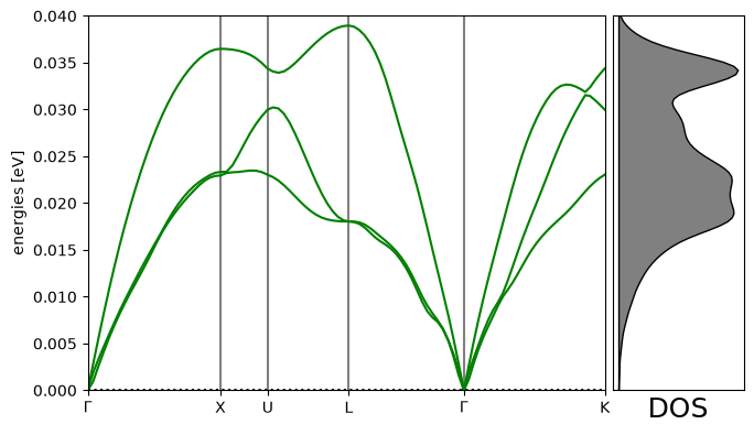
Transition States (NEBs)
Nudged elastic band calculations are among the most costly calculations we do. UMA makes these quicker!
We explore diffusion of an O adatom from an hcp to an fcc site on Pt(111).
Initial state
from ase.build import add_adsorbate, fcc111, molecule
from ase.optimize import LBFGS
from fairchem.core import FAIRChemCalculator, pretrained_mlip

predictor = pretrained_mlip.get_predict_unit("uma-s-1p2p1")
calc = FAIRChemCalculator(predictor, task_name="oc20")

# Set up your system as an ASE atoms object
initial = fcc111("Pt", (3, 3, 3), vacuum=8, periodic=True)

adsorbate = molecule("O")
add_adsorbate(initial, adsorbate, 2.0, "fcc")
initial.calc = calc

# Set up LBFGS dynamics object
opt = LBFGS(initial)
opt.run(0.05, 100)
print(initial.get_potential_energy())
WARNING:root:device was not explicitly set, using device='cuda'.
WARNING:root:Model is being compiled this might take a while for the first time
       Step     Time          Energy          fmax
LBFGS:    0 03:10:29     -141.348182        3.481489
LBFGS:    1 03:10:29     -141.726022        3.485600
LBFGS:    2 03:10:29     -142.966339        2.918310
LBFGS:    3 03:10:29     -143.656315        0.893261
LBFGS:    4 03:10:29     -143.757861        1.265100
LBFGS:    5 03:10:30     -143.833352        0.840169
LBFGS:    6 03:10:30     -143.905839        0.159555
LBFGS:    7 03:10:30     -143.910005        0.142062
LBFGS:    8 03:10:30     -143.916368        0.150821
LBFGS:    9 03:10:30     -143.921727        0.140395
LBFGS:   10 03:10:30     -143.925270        0.078516
LBFGS:   11 03:10:30     -143.927138        0.087060
LBFGS:   12 03:10:30     -143.929044        0.088637
LBFGS:   13 03:10:30     -143.931209        0.092812
LBFGS:   14 03:10:30     -143.932882        0.059820
LBFGS:   15 03:10:30     -143.933609        0.037406
-143.93360878405377
Final state
# Set up your system as an ASE atoms object
final = fcc111("Pt", (3, 3, 3), vacuum=8, periodic=True)

adsorbate = molecule("O")
add_adsorbate(final, adsorbate, 2.0, "hcp")
final.calc = FAIRChemCalculator(predictor, task_name="oc20")

# Set up LBFGS dynamics object
opt = LBFGS(final)
opt.run(0.05, 100)
print(final.get_potential_energy())
Step Time Energy fmax
LBFGS: 0 03:10:30 -141.285771 3.267078
LBFGS: 1 03:10:30 -141.646895 3.244977
LBFGS: 2 03:10:31 -142.858418 2.487965
LBFGS:    3 03:10:31     -143.364173        1.349077
LBFGS:    4 03:10:31     -143.436731        0.979108
LBFGS:    5 03:10:31     -143.570818        0.228630
LBFGS:    6 03:10:31     -143.579443        0.147465
LBFGS:    7 03:10:31     -143.582290        0.129885
LBFGS:    8 03:10:31     -143.585044        0.101465
LBFGS:    9 03:10:31     -143.586904        0.070771
LBFGS:   10 03:10:31     -143.587664        0.051365
LBFGS:   11 03:10:31     -143.588088        0.044092
-143.58808768588972
Setup and relax the band
from ase.mep import NEB

images = [initial]
for i in range(3):
    image = initial.copy()
    image.calc = FAIRChemCalculator(predictor, task_name="oc20")
    images.append(image)

images.append(final)


neb = NEB(images)
neb.interpolate()

opt = LBFGS(neb, trajectory="neb.traj")
opt.run(0.05, 100)
/home/runner/work/_tool/Python/3.12.15/x64/lib/python3.12/site-packages/ase/mep/neb.py:329: UserWarning: The default method has changed from 'aseneb' to 'improvedtangent'. The 'aseneb' method is an unpublished, custom implementation that is not recommended as it frequently results in very poor bands. Please explicitly set method='improvedtangent' to silence this warning, or set method='aseneb' if you strictly require the old behavior (results may vary). See: https://gitlab.com/ase/ase/-/merge_requests/3952
warnings.warn(
       Step     Time          Energy          fmax
LBFGS:    0 03:10:32     -143.157645        3.025170
LBFGS: 1 03:10:32 -143.322940 1.449027
LBFGS:    2 03:10:32     -143.372983        0.456653
LBFGS:    3 03:10:33     -143.384760        0.437509
LBFGS:    4 03:10:33     -143.403494        0.475290
LBFGS:    5 03:10:33     -143.420360        0.368607
LBFGS:    6 03:10:33     -143.431520        0.198334
LBFGS:    7 03:10:33     -143.436951        0.168221
LBFGS:    8 03:10:34     -143.438207        0.201689
LBFGS:    9 03:10:34     -143.439912        0.206834
LBFGS:   10 03:10:34     -143.441868        0.184462
LBFGS:   11 03:10:34     -143.443157        0.121591
LBFGS:   12 03:10:34     -143.443826        0.122842
LBFGS:   13 03:10:35     -143.444467        0.120674
LBFGS: 14 03:10:35 -143.445282 0.148221
LBFGS: 15 03:10:35 -143.446107 0.098279
LBFGS: 16 03:10:35 -143.446622 0.064176
LBFGS: 17 03:10:36 -143.446975 0.062956
LBFGS: 18 03:10:36 -143.447430 0.107954
LBFGS: 19 03:10:36 -143.447968 0.096170
LBFGS: 20 03:10:37 -143.448326 0.048750
np.True_from ase.mep import NEBTools
NEBTools(neb.images).plot_band();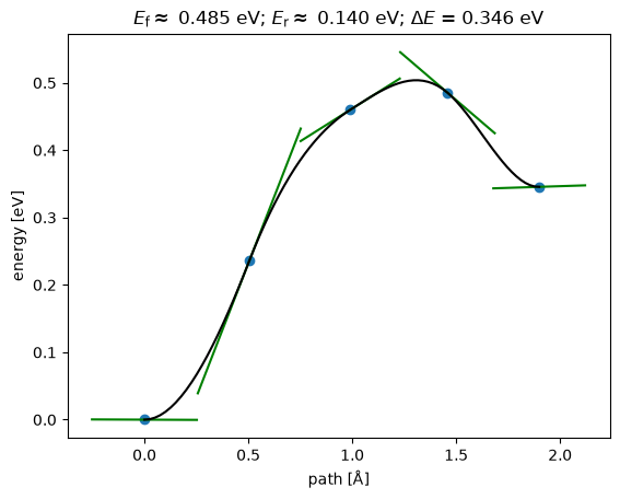
This could be a good initial guess to initialize an NEB in DFT.
Ideas for things you can do with UMA
Advanced applications
These take a while to run.
AdsorbML
It is so cheap to run these calculations that we can screen a broad range of adsorbate sites and rank them in stability. The AdsorbML approach automates this. This takes quite a while to run here, and we don’t do it in the workshop.
Expert adsorption energies
This tutorial reproduces Fig 6b from the following paper: Zhou, Jing, et al. “Enhanced Catalytic Activity of Bimetallic Ordered Catalysts for Nitrogen Reduction Reaction by Perturbation of Scaling Relations.” ACS Catalysis 134 (2023): 2190-2201 (Zhou & others (2023)).
This takes up to an hour with a GPU, and much longer with a CPU.
CatTsunami
The CatTsunami tutorial is an example of enumerating initial and final states, and computing reaction paths between them with UMA.
Acknowledgments
This tutorial was originally compiled by John Kitchin (CMU) for the NAM29 catalysis tutorial session, using a variety of resources from the FAIR chemistry repository.
- Musielewicz, J., Wang, X., Tian, T., & Ulissi, Z. (2022). FINETUNA: fine-tuning accelerated molecular simulations. Machine Learning: Science and Technology, 3(3), 03LT01. 10.1088/2632-2153/ac8fe0
- Wang, X., Musielewicz, J., Tran, R., Ethirajan, S. K., Fu, X., Mera, H., Kitchin, J. R., Kurchin, R. C., & Ulissi, Z. W. (2024). Generalization of graph-based active learning relaxation strategies across materials. Machine Learning: Science and Technology, 5(2), 025018. 10.1088/2632-2153/ad37f0
- Wander, B., Shuaibi, M., Kitchin, J. R., Ulissi, Z. W., & Zitnick, C. L. (2024). CatTSunami: Accelerating Transition State Energy Calculations with Pre-trained Graph Neural Networks. ACS Catalysis. 10.1021/acscatal.4c04272
- Vibrational Free Energy Estimation with Machine-Learned Interatomic Potentials. (2024). The Journal of Physical Chemistry C. 10.1021/acs.jpcc.4c07477
- Zhou, J., & others. (2023). Enhanced Catalytic Activity of Bimetallic Ordered Catalysts for Nitrogen Reduction Reaction by Perturbation of Scaling Relations. 10.1021/acscatal.2c05877