| Property | Value |
|---|---|
| Difficulty | Beginner |
| Time | 15-30 minutes |
| Prerequisites | Basic Python, familiarity with ASE |
| Goal | Calculate adsorption energies using UMA models |
To introduce OCP we start with using it to calculate adsorption energies for a simple, atomic adsorbate where we specify the site we want to the adsorption energy for. Conceptually, you do this like you would do it with density functional theory. You create a slab model for the surface, place an adsorbate on it as an initial guess, run a relaxation to get the lowest energy geometry, and then compute the adsorption energy using reference states for the adsorbate.
Intro to Adsorption energies
Adsorption energies are always a reaction energy (an adsorbed species relative to some implied combination of reactants). There are many common schemes in the catalysis literature.
For example, you may want the adsorption energy of oxygen, and you might compute that from this reaction:
1/2 O2 + slab -> slab-ODFT has known errors with the energy of a gas-phase O2 molecule, so it’s more common to compute this energy relative to a linear combination of H2O and H2. The suggested reference scheme for consistency with OC20 is a reaction
x CO + (x + y/2 - z) H2 + (z-x) H2O + w/2 N2 + * -> CxHyOzNw*Here, x=y=w=0, z=1, so the reaction ends up as
-H2 + H2O + * -> O*or alternatively,
H2O + * -> O* + H2It is possible through thermodynamic cycles to compute other reactions. If we can look up rH1 below and compute rH2
H2 + 1/2 O2 -> H2O  re1 = -3.03 eV, from exp
H2O + * -> O* + H2  re2  # Get from UMA
Then, the adsorption energy for
1/2O2 + * -> O*is just re1 + re2.
Based on https://atct.anl.gov/Thermochemical Data/version 1.118/species/?species_number=986, the formation energy of water is about -3.03 eV at standard state experimentally. You could also compute this using DFT, but you would probably get the wrong answer for this.
The first step is getting a checkpoint for the model we want to use. UMA is currently the state-of-the-art model and will provide total energy estimates at the RPBE level of theory if you use the “OC20” task.
Need to install fairchem-core or get UMA access or getting permissions/401 errors?
Install the necessary packages using pip, uv etc
! pip install fairchem-core fairchem-data-oc fairchem-applications-cattsunamiGet access to any necessary huggingface gated models
Get and login to your Huggingface account
Request access to https://
huggingface .co /facebook /UMA Create a Huggingface token at https://
huggingface .co /settings /tokens/ with the permission “Permissions: Read access to contents of all public gated repos you can access” Add the token as an environment variable using
huggingface-cli loginor by setting the HF_TOKEN environment variable.
# Login using the huggingface-cli utility
! huggingface-cli login

# alternatively,
import os
os.environ['HF_TOKEN'] = 'MY_TOKEN'
If you find your kernel is crashing, it probably means you have exceeded the allowed amount of memory. This checkpoint works fine in this example, but it may crash your kernel if you use it in the NRR example.
This next cell will automatically download the checkpoint from huggingface and load it.
from __future__ import annotations

from fairchem.core import FAIRChemCalculator, pretrained_mlip

predictor = pretrained_mlip.get_predict_unit("uma-s-1p2p1")
calc = FAIRChemCalculator(predictor, task_name="oc20")
Warp 1.18.0 initialized:
CUDA Toolkit 13.4, Driver 13.1
Devices:
"cpu" : "x86_64"
"cuda:0" : "Tesla T4" (16 GiB, sm_75, mempool enabled)
Kernel cache:
/home/runner/.cache/warp/1.18.0
WARNING:root:device was not explicitly set, using device='cuda'.
Next we can build a slab with an adsorbate on it. Here we use the ASE module to build a Pt slab. We use the experimental lattice constant that is the default. This can introduce some small errors with DFT since the lattice constant can differ by a few percent, and it is common to use DFT lattice constants. In this example, we do not constrain any layers.
from ase.build import add_adsorbate, fcc111
from ase.optimize import BFGS
# reference energies from a linear combination of H2O/N2/CO/H2!
atomic_reference_energies = {
"H": -3.477,
"N": -8.083,
"O": -7.204,
"C": -7.282,
}
re1 = -3.03
slab = fcc111("Pt", size=(2, 2, 5), vacuum=20.0)
slab.pbc = True
adslab = slab.copy()
add_adsorbate(adslab, "O", height=1.2, position="fcc")
slab.set_calculator(calc)
opt = BFGS(slab)
opt.run(fmax=0.05, steps=100)
slab_e = slab.get_potential_energy()
adslab.set_calculator(calc)
opt = BFGS(adslab)
opt.run(fmax=0.05, steps=100)
adslab_e = adslab.get_potential_energy()
# Energy for ((H2O-H2) + * -> *O) + (H2 + 1/2O2 -> H2) leads to 1/2O2 + * -> *O!
adslab_e - slab_e - atomic_reference_energies["O"] + re1/tmp/ipykernel_9020/3752951811.py:17: FutureWarning: Please use atoms.calc = calc
slab.set_calculator(calc)
WARNING:root:Model is being compiled this might take a while for the first time
W1007 02:52:48.082000 9020 site-packages/torch/_logging/_internal.py:1345] [0/0] Profiler record function <class 'torch.autograd.profiler.record_function'> will be ignored
      Step     Time          Energy          fmax
BFGS:    0 02:53:39     -104.713230        0.695698
BFGS:    1 02:53:40     -104.770833        0.592989
BFGS:    2 02:53:40     -104.910089        0.340089
BFGS:    3 02:53:40     -104.937705        0.411463
BFGS:    4 02:53:40     -105.009224        0.454733
BFGS:    5 02:53:40     -105.068379        0.352806
BFGS:    6 02:53:40     -105.105354        0.173377
/tmp/ipykernel_9020/3752951811.py:22: FutureWarning: Please use atoms.calc = calc
  adslab.set_calculator(calc)
WARNING:root:The UMA fast path (merge_mole + compile) is only available for fixed composition, task, charge, and spin. This is optimized for MD applications. Falling back to a less optimized version for subsequent evaluations. Reason: 'Compositions differ from merged model'.
Use inference_settings='batch' for heterogeneous batched evaluations.
BFGS: 7 02:53:40 -105.116035 0.042057
      Step     Time          Energy          fmax
BFGS:    0 02:53:46     -110.098582        1.709169
BFGS:    1 02:53:46     -110.275966        0.961389
BFGS:    2 02:53:47     -110.420420        0.724063
BFGS:    3 02:53:47     -110.468239        0.788379
BFGS:    4 02:53:47     -110.569492        0.640721
BFGS:    5 02:53:47     -110.633821        0.473712
BFGS:    6 02:53:47     -110.685971        0.559150
BFGS:    7 02:53:48     -110.731266        0.612418
BFGS: 8 02:53:48 -110.762440 0.457342
BFGS: 9 02:53:48 -110.776662 0.240128
BFGS: 10 02:53:48 -110.780698 0.109504
BFGS: 11 02:53:48 -110.781687 0.093773
BFGS: 12 02:53:49 -110.782524 0.057397
BFGS: 13 02:53:49 -110.783130 0.043503
-1.4930957656456978It is good practice to look at your geometries to make sure they are what you expect.
import matplotlib.pyplot as plt
from ase.visualize.plot import plot_atoms

fig, axs = plt.subplots(1, 2)
plot_atoms(slab, axs[0])
plot_atoms(slab, axs[1], rotation=("-90x"))
axs[0].set_axis_off()
axs[1].set_axis_off()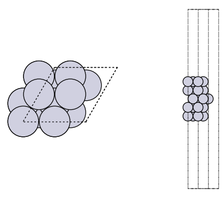
import matplotlib.pyplot as plt
from ase.visualize.plot import plot_atoms

fig, axs = plt.subplots(1, 2)
plot_atoms(adslab, axs[0])
plot_atoms(adslab, axs[1], rotation=("-90x"))
axs[0].set_axis_off()
axs[1].set_axis_off()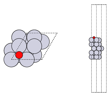
How did we do? We need a reference point. In the paper below, there is an atomic adsorption energy for O on Pt(111) of about -4.264 eV. This is for the reaction O + * -> O*. To convert this to the dissociative adsorption energy, we have to add the reaction:
1/2 O2 -> O D = 2.58 eV (expt)to get a comparable energy of about -1.68 eV. There is about ~0.2 eV difference (we predicted -1.47 eV above, and the reference comparison is -1.68 eV) to account for. The biggest difference is likely due to the differences in exchange-correlation functional. The reference data used the PBE functional, and eSCN was trained on RPBE data. To additional places where there are differences include:
Difference in lattice constant
The reference energy used for the experiment references. These can differ by up to 0.5 eV from comparable DFT calculations.
How many layers are relaxed in the calculation
Some of these differences tend to be systematic, and you can calibrate and correct these, especially if you can augment these with your own DFT calculations.
See convergence study for some additional studies of factors that influence this number.
Exercises
Explore the effect of the lattice constant on the adsorption energy.
Try different sites, including the bridge and top sites. Compare the energies, and inspect the resulting geometries.
Trends in adsorption energies across metals.
Xu, Z., & Kitchin, J. R. (2014). Probing the coverage dependence of site and adsorbate configurational correlations on (111) surfaces of late transition metals. J. Phys. Chem. C, 118(44), 25597–25602. Xu & Kitchin (2014)
These are atomic adsorption energies:
O + * -> O*We have to do some work to get comparable numbers from OCP
H2 + 1/2 O2 -> H2O  re1 = -3.03 eV
H2O + * -> O* + H2  re2   # Get from UMA
O -> 1/2 O2         re3 = -2.58 eV
Then, the adsorption energy for
O + * -> O*is just re1 + re2 + re3.
Here we just look at the fcc site on Pt. First, we get the data stored in the paper.
Next we get the structures and compute their energies. Some subtle points are that we have to account for stoichiometry, and normalize the adsorption energy by the number of oxygens.
First we get a reference energy from the paper (PBE, 0.25 ML O on Pt(111)).
import json

with open("energies.json") as f:
    edata = json.load(f)

with open("structures.json") as f:
    sdata = json.load(f)

edata["Pt"]["O"]["fcc"]["0.25"]-4.263842000000002Next, we load data from the SI to get the geometry to start from.
with open("structures.json") as f:
    s = json.load(f)

sfcc = s["Pt"]["O"]["fcc"]["0.25"]
Next, we construct the atomic geometry, run the geometry optimization, and compute the energy.
re3 = -2.58  # O -> 1/2 O2         re3 = -2.58 eV

from ase import Atoms

adslab = Atoms(sfcc["symbols"], positions=sfcc["pos"], cell=sfcc["cell"], pbc=True)

# Grab just the metal surface atoms
slab = adslab[adslab.arrays["numbers"] == adslab.arrays["numbers"][0]]
adsorbates = adslab[~(adslab.arrays["numbers"] == adslab.arrays["numbers"][0])]
slab.set_calculator(calc)
opt = BFGS(slab)
opt.run(fmax=0.05, steps=100)

adslab.set_calculator(calc)
opt = BFGS(adslab)

opt.run(fmax=0.05, steps=100)
re2 = (
    adslab.get_potential_energy()
    - slab.get_potential_energy()
    - sum([atomic_reference_energies[x] for x in adsorbates.get_chemical_symbols()])
)

nO = 0
for atom in adslab:
    if atom.symbol == "O":
        nO += 1
        re2 += re1 + re3

print(re2 / nO)
/tmp/ipykernel_9020/647904475.py:10: FutureWarning: Please use atoms.calc = calc
slab.set_calculator(calc)
      Step     Time          Energy          fmax
BFGS:    0 02:53:52      -82.875792        1.001622
BFGS:    1 02:53:52      -82.933706        0.753713
BFGS: 2 02:53:53 -83.029081 0.343665
BFGS: 3 02:53:53 -83.033631 0.315207
BFGS: 4 02:53:53 -83.043724 0.217719
BFGS:    5 02:53:53      -83.048510        0.144969
BFGS:    6 02:53:53      -83.051139        0.085603
BFGS:    7 02:53:54      -83.052235        0.080541
BFGS:    8 02:53:54      -83.053002        0.071009
BFGS:    9 02:53:54      -83.053265        0.042013
      Step     Time          Energy          fmax
BFGS:    0 02:53:54      -88.766845        0.297396
/tmp/ipykernel_9020/647904475.py:14: FutureWarning: Please use atoms.calc = calc
  adslab.set_calculator(calc)
BFGS: 1 02:53:54 -88.770224 0.257427
BFGS:    2 02:53:54      -88.780027        0.098767
BFGS:    3 02:53:55      -88.781393        0.101431
BFGS: 4 02:53:55 -88.785247 0.121376
BFGS: 5 02:53:55 -88.787298 0.095675
BFGS: 6 02:53:55 -88.788632 0.063880
BFGS:    7 02:53:56      -88.789399        0.055449
BFGS:    8 02:53:56      -88.789993        0.047874
-4.142727727566048
Site correlations
This cell reproduces a portion of a figure in the paper. We compare oxygen adsorption energies in the fcc and hcp sites across metals and coverages. These adsorption energies are highly correlated with each other because the adsorption sites are so similar.
At higher coverages, the agreement is not as good. This is likely because the model is extrapolating and needs to be fine-tuned.
import time

from tqdm import tqdm

t0 = time.time()

data = {"fcc": [], "hcp": []}

refdata = {"fcc": [], "hcp": []}


for metal in ["Cu", "Ag", "Pd", "Pt", "Rh", "Ir"]:
    print(metal)
    for site in ["fcc", "hcp"]:
        for adsorbate in ["O"]:
            for coverage in tqdm(["0.25"]):

                entry = s[metal][adsorbate][site][coverage]

                adslab = Atoms(
                    entry["symbols"],
                    positions=entry["pos"],
                    cell=entry["cell"],
                    pbc=True,
                )

                # Grab just the metal surface atoms
                adsorbates = adslab[
                    ~(adslab.arrays["numbers"] == adslab.arrays["numbers"][0])
                ]

                slab = adslab[adslab.arrays["numbers"] == adslab.arrays["numbers"][0]]
                slab.set_calculator(calc)
                opt = BFGS(slab)
                opt.run(fmax=0.05, steps=100)

                adslab.set_calculator(calc)
                opt = BFGS(adslab)
                opt.run(fmax=0.05, steps=100)

                re2 = (
                    adslab.get_potential_energy()
                    - slab.get_potential_energy()
                    - sum(
                        [
                            atomic_reference_energies[x]
                            for x in adsorbates.get_chemical_symbols()
                        ]
                    )
                )

                nO = 0
                for atom in adslab:
                    if atom.symbol == "O":
                        nO += 1
                        re2 += re1 + re3

                data[site] += [re2 / nO]
                refdata[site] += [edata[metal][adsorbate][site][coverage]]

f"Elapsed time = {time.time() - t0} seconds"
Cu
0%| | 0/1 [00:00<?, ?it/s] Step Time Energy fmax
BFGS: 0 02:53:56 -48.900179 0.640047
BFGS: 1 02:53:56 -48.922875 0.535702
/tmp/ipykernel_9020/1356342052.py:33: FutureWarning: Please use atoms.calc = calc
  slab.set_calculator(calc)
BFGS:    2 02:53:56      -48.987830        0.278368
BFGS:    3 02:53:56      -48.990214        0.248664
BFGS:    4 02:53:57      -48.996771        0.151935
BFGS:    5 02:53:57      -49.001688        0.134448
BFGS:    6 02:53:57      -49.004634        0.067513
BFGS:    7 02:53:57      -49.005324        0.049306
/tmp/ipykernel_9020/1356342052.py:37: FutureWarning: Please use atoms.calc = calc
  adslab.set_calculator(calc)
      Step     Time          Energy          fmax
BFGS:    0 02:53:57      -55.218070        0.302093
BFGS:    1 02:53:57      -55.220112        0.247387
BFGS:    2 02:53:58      -55.227359        0.151302
BFGS:    3 02:53:58      -55.229153        0.148929
BFGS:    4 02:53:58      -55.232173        0.091641
BFGS:    5 02:53:58      -55.233780        0.078586
BFGS:    6 02:53:58      -55.235011        0.078970
BFGS:    7 02:53:58      -55.236088        0.099330
BFGS:    8 02:53:59      -55.237336        0.093224
BFGS:    9 02:53:59      -55.238151        0.053164
100%|██████████| 1/1 [00:03<00:00, 3.31s/it]100%|██████████| 1/1 [00:03<00:00, 3.31s/it]
BFGS: 10 02:53:59 -55.238500 0.041211
0%| | 0/1 [00:00<?, ?it/s] Step Time Energy fmax
BFGS: 0 02:53:59 -48.924787 0.554787
BFGS: 1 02:53:59 -48.942464 0.470220
BFGS: 2 02:54:00 -48.996418 0.215336
BFGS: 3 02:54:00 -48.997677 0.194299
BFGS: 4 02:54:00 -49.003507 0.083910
BFGS:    5 02:54:00      -49.005257        0.064526
BFGS:    6 02:54:00      -49.005839        0.042565
      Step     Time          Energy          fmax
BFGS:    0 02:54:01      -55.116423        0.283250
BFGS:    1 02:54:01      -55.118140        0.228270
BFGS: 2 02:54:01 -55.123705 0.148243
BFGS: 3 02:54:01 -55.125335 0.153679
BFGS:    4 02:54:01      -55.128601        0.101045
BFGS:    5 02:54:02      -55.129937        0.061993
BFGS:    6 02:54:02      -55.130646        0.052161
BFGS:    7 02:54:02      -55.131257        0.073539
BFGS: 8 02:54:02 -55.132125 0.080354
BFGS:    9 02:54:02      -55.132811        0.052464
BFGS:   10 02:54:02      -55.133081        0.029269
100%|██████████| 1/1 [00:03<00:00, 3.33s/it]100%|██████████| 1/1 [00:03<00:00, 3.33s/it]
Ag
0%| | 0/1 [00:00<?, ?it/s] Step Time Energy fmax
BFGS: 0 02:54:03 -33.031602 0.626106
BFGS: 1 02:54:03 -33.050396 0.544534
BFGS: 2 02:54:03 -33.117862 0.175300
BFGS: 3 02:54:03 -33.119736 0.160487
BFGS: 4 02:54:03 -33.121179 0.145178
BFGS: 5 02:54:03 -33.123868 0.114213
BFGS: 6 02:54:04 -33.127505 0.105987
BFGS: 7 02:54:04 -33.130241 0.068348
BFGS: 8 02:54:04 -33.131083 0.031900
      Step     Time          Energy          fmax
BFGS:    0 02:54:04      -38.192075        0.102268
BFGS:    1 02:54:04      -38.193078        0.099456
BFGS: 2 02:54:04 -38.203696 0.090586
BFGS: 3 02:54:05 -38.204613 0.091026
BFGS: 4 02:54:05 -38.207030 0.090028
BFGS: 5 02:54:05 -38.209186 0.077640
BFGS:    6 02:54:05      -38.210986        0.071168
BFGS:    7 02:54:05      -38.211907        0.063849
100%|██████████| 1/1 [00:03<00:00, 3.20s/it]100%|██████████| 1/1 [00:03<00:00, 3.20s/it]
BFGS: 8 02:54:06 -38.212367 0.043668
0%| | 0/1 [00:00<?, ?it/s] Step Time Energy fmax
BFGS: 0 02:54:06 -33.054096 0.549953
BFGS: 1 02:54:06 -33.068314 0.483648
BFGS: 2 02:54:06 -33.123290 0.132357
BFGS:    3 02:54:06      -33.124235        0.121002
BFGS:    4 02:54:07      -33.125328        0.105056
BFGS:    5 02:54:07      -33.127116        0.077530
BFGS:    6 02:54:07      -33.129497        0.074666
BFGS:    7 02:54:07      -33.130956        0.042329
      Step     Time          Energy          fmax
BFGS:    0 02:54:07      -38.108665        0.095167
BFGS: 1 02:54:07 -38.109542 0.090901
BFGS: 2 02:54:08 -38.119361 0.103904
BFGS: 3 02:54:08 -38.120376 0.087527
BFGS:    4 02:54:08      -38.122369        0.078400
BFGS:    5 02:54:08      -38.123732        0.068548
BFGS:    6 02:54:08      -38.124838        0.063109
BFGS:    7 02:54:09      -38.125562        0.066961
100%|██████████| 1/1 [00:03<00:00, 3.23s/it]100%|██████████| 1/1 [00:03<00:00, 3.24s/it]
BFGS:    8 02:54:09      -38.126100        0.049381
Pd
0%| | 0/1 [00:00<?, ?it/s] Step Time Energy fmax
BFGS: 0 02:54:09 -70.160649 0.637749
BFGS: 1 02:54:09 -70.185883 0.514166
BFGS:    2 02:54:09      -70.238641        0.202178
BFGS:    3 02:54:10      -70.240303        0.193176
BFGS:    4 02:54:10      -70.247439        0.136878
BFGS:    5 02:54:10      -70.250340        0.103755
BFGS:    6 02:54:10      -70.252112        0.071685
BFGS:    7 02:54:10      -70.252969        0.062166
BFGS:    8 02:54:10      -70.253731        0.040143
      Step     Time          Energy          fmax
BFGS:    0 02:54:11      -76.126861        0.226787
BFGS:    1 02:54:11      -76.129898        0.202917
BFGS:    2 02:54:11      -76.143234        0.150963
BFGS: 3 02:54:11 -76.144931 0.125403
BFGS:    4 02:54:11      -76.149177        0.128495
BFGS:    5 02:54:12      -76.152035        0.102057
BFGS:    6 02:54:12      -76.154435        0.097338
BFGS:    7 02:54:12      -76.155611        0.079966
100%|██████████| 1/1 [00:03<00:00, 3.37s/it]100%|██████████| 1/1 [00:03<00:00, 3.38s/it]
BFGS: 8 02:54:12 -76.156308 0.049423
0%| | 0/1 [00:00<?, ?it/s] Step Time Energy fmax
BFGS: 0 02:54:13 -70.193620 0.457899
BFGS: 1 02:54:13 -70.207966 0.375579
BFGS:    2 02:54:13      -70.243018        0.185785
BFGS:    3 02:54:13      -70.244247        0.172444
BFGS:    4 02:54:13      -70.251214        0.078480
BFGS:    5 02:54:13      -70.252103        0.072906
BFGS: 6 02:54:13 -70.252951 0.052548
BFGS: 7 02:54:14 -70.253591 0.041705
      Step     Time          Energy          fmax
BFGS:    0 02:54:14      -75.926065        0.184330
BFGS:    1 02:54:14      -75.929168        0.164894
BFGS:    2 02:54:14      -75.939950        0.164991
BFGS: 3 02:54:14 -75.941728 0.149947
BFGS: 4 02:54:15 -75.947054 0.125715
BFGS: 5 02:54:15 -75.949697 0.117586
BFGS: 6 02:54:15 -75.951841 0.087773
BFGS: 7 02:54:15 -75.952947 0.071385
100%|██████████| 1/1 [00:03<00:00, 3.42s/it]100%|██████████| 1/1 [00:03<00:00, 3.42s/it]
BFGS:    8 02:54:16      -75.953493        0.035904
Pt
0%| | 0/1 [00:00<?, ?it/s] Step Time Energy fmax
BFGS: 0 02:54:16 -82.875791 1.001622
BFGS: 1 02:54:16 -82.933706 0.753713
BFGS: 2 02:54:16 -83.029080 0.343665
BFGS: 3 02:54:17 -83.033633 0.315206
BFGS: 4 02:54:17 -83.043723 0.217706
BFGS: 5 02:54:17 -83.048510 0.144962
BFGS: 6 02:54:17 -83.051140 0.085608
BFGS: 7 02:54:18 -83.052235 0.080542
BFGS: 8 02:54:18 -83.053001 0.071028
BFGS:    9 02:54:18      -83.053265        0.042015
      Step     Time          Energy          fmax
BFGS:    0 02:54:18      -88.766845        0.297396
BFGS:    1 02:54:18      -88.770225        0.257428
BFGS:    2 02:54:19      -88.780027        0.098767
BFGS:    3 02:54:19      -88.781393        0.101431
BFGS:    4 02:54:19      -88.785248        0.121376
BFGS:    5 02:54:19      -88.787298        0.095674
BFGS:    6 02:54:19      -88.788633        0.063882
BFGS:    7 02:54:19      -88.789397        0.055461
100%|██████████| 1/1 [00:03<00:00, 3.72s/it]100%|██████████| 1/1 [00:03<00:00, 3.72s/it]
BFGS: 8 02:54:19 -88.789993 0.047876
0%| | 0/1 [00:00<?, ?it/s] Step Time Energy fmax
BFGS: 0 02:54:20 -82.961449 0.691639
BFGS: 1 02:54:20 -82.988845 0.558769
BFGS: 2 02:54:20 -83.043712 0.215073
BFGS: 3 02:54:20 -83.045355 0.197420
BFGS: 4 02:54:21 -83.051504 0.074777
BFGS: 5 02:54:21 -83.052048 0.063785
BFGS:    6 02:54:21      -83.053208        0.026290
      Step     Time          Energy          fmax
BFGS:    0 02:54:21      -88.381492        0.203486
BFGS: 1 02:54:21 -88.384463 0.178577
BFGS: 2 02:54:22 -88.394170 0.103812
BFGS: 3 02:54:22 -88.395737 0.114229
BFGS: 4 02:54:22 -88.400247 0.112557
BFGS: 5 02:54:22 -88.402088 0.091293
BFGS: 6 02:54:23 -88.403049 0.065532
BFGS: 7 02:54:23 -88.403428 0.050622
BFGS: 8 02:54:23 -88.403755 0.031911
100%|██████████| 1/1 [00:04<00:00, 4.02s/it]100%|██████████| 1/1 [00:04<00:00, 4.02s/it]
Rh
0%| | 0/1 [00:00<?, ?it/s] Step Time Energy fmax
BFGS: 0 02:54:24 -100.178311 0.695372
BFGS: 1 02:54:24 -100.205471 0.605778
BFGS:    2 02:54:24     -100.274451        0.188597
BFGS:    3 02:54:24     -100.277839        0.131927
BFGS:    4 02:54:24     -100.286140        0.092537
BFGS:    5 02:54:25     -100.288426        0.063499
BFGS:    6 02:54:25     -100.289378        0.054370
BFGS:    7 02:54:25     -100.290038        0.049018
      Step     Time          Energy          fmax
BFGS:    0 02:54:25     -106.914346        0.219023
BFGS: 1 02:54:25 -106.918825 0.183724
BFGS: 2 02:54:26 -106.927824 0.092936
BFGS: 3 02:54:26 -106.928192 0.080083
100%|██████████| 1/1 [00:02<00:00, 2.83s/it]100%|██████████| 1/1 [00:02<00:00, 2.84s/it]
BFGS: 4 02:54:26 -106.929645 0.038195
0%| | 0/1 [00:00<?, ?it/s] Step Time Energy fmax
BFGS: 0 02:54:27 -100.158081 0.745159
BFGS: 1 02:54:27 -100.191364 0.622306
BFGS: 2 02:54:27 -100.275626 0.242940
BFGS: 3 02:54:27 -100.278649 0.184961
BFGS: 4 02:54:27 -100.287116 0.079709
BFGS:    5 02:54:28     -100.288603        0.075170
BFGS:    6 02:54:28     -100.289527        0.057056
BFGS: 7 02:54:28 -100.290225 0.053811
BFGS:    8 02:54:28     -100.290732        0.043520
      Step     Time          Energy          fmax
BFGS:    0 02:54:28     -106.879013        0.258383
BFGS:    1 02:54:29     -106.884265        0.206354
BFGS:    2 02:54:29     -106.894906        0.097876
BFGS:    3 02:54:29     -106.895276        0.085970
BFGS:    4 02:54:29     -106.896699        0.029152
100%|██████████| 1/1 [00:03<00:00, 3.07s/it]100%|██████████| 1/1 [00:03<00:00, 3.07s/it]
Ir
0%| | 0/1 [00:00<?, ?it/s] Step Time Energy fmax
BFGS: 0 02:54:30 -124.228111 1.174836
BFGS: 1 02:54:30 -124.302341 0.929052
BFGS: 2 02:54:30 -124.414172 0.175909
BFGS: 3 02:54:30 -124.417641 0.151208
BFGS: 4 02:54:30 -124.423797 0.050082
BFGS:    5 02:54:30     -124.424160        0.045537
      Step     Time          Energy          fmax
BFGS:    0 02:54:31     -130.607362        0.412837
BFGS: 1 02:54:31 -130.622208 0.291773
BFGS: 2 02:54:31 -130.641299 0.174542
BFGS: 3 02:54:31 -130.642828 0.164442
BFGS: 4 02:54:32 -130.651892 0.072379
BFGS: 5 02:54:32 -130.652869 0.088889
BFGS: 6 02:54:32 -130.654270 0.083062
100%|██████████| 1/1 [00:02<00:00, 2.90s/it]100%|██████████| 1/1 [00:02<00:00, 2.91s/it]
BFGS: 7 02:54:32 -130.655170 0.047622
0%| | 0/1 [00:00<?, ?it/s] Step Time Energy fmax
BFGS: 0 02:54:33 -124.221688 1.137424
BFGS: 1 02:54:33 -124.303038 0.897451
BFGS: 2 02:54:33 -124.414782 0.205397
BFGS: 3 02:54:33 -124.417803 0.206964
BFGS: 4 02:54:33 -124.423751 0.101231
BFGS: 5 02:54:34 -124.424199 0.068196
BFGS: 6 02:54:34 -124.424826 0.037612
      Step     Time          Energy          fmax
BFGS:    0 02:54:34     -130.494954        0.471648
BFGS:    1 02:54:34     -130.510728        0.339461
BFGS: 2 02:54:35 -130.528898 0.157428
BFGS: 3 02:54:35 -130.529651 0.147624
BFGS: 4 02:54:35 -130.534002 0.056971
BFGS: 5 02:54:35 -130.534285 0.060613
100%|██████████| 1/1 [00:03<00:00, 3.43s/it]100%|██████████| 1/1 [00:03<00:00, 3.43s/it]BFGS: 6 02:54:36 -130.534865 0.037244
'Elapsed time = 39.943995237350464 seconds'First, we compare the computed data and reference data. There is a systematic difference of about 0.5 eV due to the difference between RPBE and PBE functionals, and other subtle differences like lattice constant differences and reference energy differences. This is pretty typical, and an expected deviation.
plt.plot(refdata["fcc"], data["fcc"], "r.", label="fcc")
plt.plot(refdata["hcp"], data["hcp"], "b.", label="hcp")
plt.plot([-5.5, -3.5], [-5.5, -3.5], "k-")
plt.xlabel("Ref. data (DFT)")
plt.ylabel("UMA-OC20 prediction");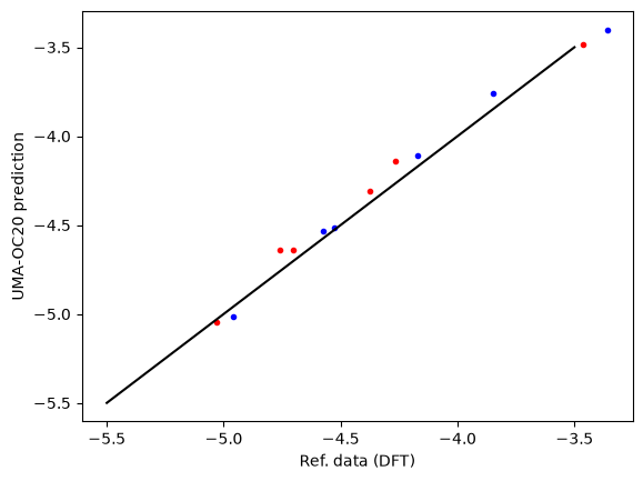
Next we compare the correlation between the hcp and fcc sites. Here we see the same trends. The data falls below the parity line because the hcp sites tend to be a little weaker binding than the fcc sites.
plt.plot(refdata["hcp"], refdata["fcc"], "r.")
plt.plot(data["hcp"], data["fcc"], ".")
plt.plot([-6, -1], [-6, -1], "k-")
plt.xlabel("$H_{ads, hcp}$")
plt.ylabel("$H_{ads, fcc}$")
plt.legend(["DFT (PBE)", "UMA-OC20"]);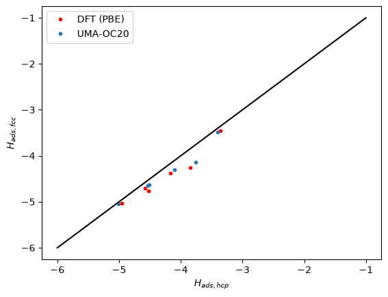
Exercises
You can also explore a few other adsorbates: C, H, N.
Explore the higher coverages. The deviations from the reference data are expected to be higher, but relative differences tend to be better. You probably need fine tuning to improve this performance. This data set doesn’t have forces though, so it isn’t practical to do it here.
Next steps
In the next step, we consider some more complex adsorbates in nitrogen reduction, and how we can leverage OCP to automate the search for the most stable adsorbate geometry. See the next step.
Convergence study
In the adsorption energies section we discussed some possible reasons we might see a discrepancy. Here we investigate some factors that impact the computed energies.
In this section, the energies refer to the reaction 1/2 O2 -> O*.
Effects of number of layers
Slab thickness could be a factor. Here we relax the whole slab, and see by about 4 layers the energy is converged to ~0.02 eV.
for nlayers in [3, 4, 5, 6, 7, 8]:
    slab = fcc111("Pt", size=(2, 2, nlayers), vacuum=10.0)

    slab.pbc = True
    slab.set_calculator(calc)
    opt_slab = BFGS(slab, logfile=None)
    opt_slab.run(fmax=0.05, steps=100)
    slab_e = slab.get_potential_energy()

    adslab = slab.copy()
    add_adsorbate(adslab, "O", height=1.2, position="fcc")

    adslab.pbc = True
    adslab.set_calculator(calc)
    opt_adslab = BFGS(adslab, logfile=None)
    opt_adslab.run(fmax=0.05, steps=100)
    adslab_e = adslab.get_potential_energy()

    print(
        f"nlayers = {nlayers}: {adslab_e - slab_e - atomic_reference_energies['O'] + re1:1.2f} eV"
    )
/tmp/ipykernel_9020/338101817.py:5: FutureWarning: Please use atoms.calc = calc
slab.set_calculator(calc)
/tmp/ipykernel_9020/338101817.py:14: FutureWarning: Please use atoms.calc = calc
  adslab.set_calculator(calc)
nlayers = 3: -1.61 eV
nlayers = 4: -1.47 eV
nlayers = 5: -1.49 eV
nlayers = 6: -1.50 eV
nlayers = 7: -1.50 eV
nlayers = 8: -1.51 eV
Effects of relaxation
It is common to only relax a few layers, and constrain lower layers to bulk coordinates. We do that here. We only relax the adsorbate and the top layer.
This has a small effect (0.1 eV).
from ase.constraints import FixAtoms

for nlayers in [3, 4, 5, 6, 7, 8]:
    slab = fcc111("Pt", size=(2, 2, nlayers), vacuum=10.0)

    slab.set_constraint(FixAtoms(mask=[atom.tag > 1 for atom in slab]))
    slab.pbc = True
    slab.set_calculator(calc)
    opt_slab = BFGS(slab, logfile=None)
    opt_slab.run(fmax=0.05, steps=100)
    slab_e = slab.get_potential_energy()

    adslab = slab.copy()
    add_adsorbate(adslab, "O", height=1.2, position="fcc")

    adslab.set_constraint(FixAtoms(mask=[atom.tag > 1 for atom in adslab]))
    adslab.pbc = True
    adslab.set_calculator(calc)
    opt_adslab = BFGS(adslab, logfile=None)
    opt_adslab.run(fmax=0.05, steps=100)
    adslab_e = adslab.get_potential_energy()

    print(
        f"nlayers = {nlayers}: {adslab_e - slab_e - atomic_reference_energies['O'] + re1:1.2f} eV"
    )
/tmp/ipykernel_9020/1426773950.py:8: FutureWarning: Please use atoms.calc = calc
slab.set_calculator(calc)
/tmp/ipykernel_9020/1426773950.py:18: FutureWarning: Please use atoms.calc = calc
  adslab.set_calculator(calc)
nlayers = 3: -1.51 eV
nlayers = 4: -1.37 eV
nlayers = 5: -1.39 eV
nlayers = 6: -1.40 eV
nlayers = 7: -1.40 eV
nlayers = 8: -1.40 eV
Unit cell size
Coverage effects are quite noticeable with oxygen. Here we consider larger unit cells. This effect is large, and the results don’t look right, usually adsorption energies get more favorable at lower coverage, not less. This suggests fine-tuning could be important even at low coverages.
for size in [1, 2, 3, 4, 5]:

    slab = fcc111("Pt", size=(size, size, 5), vacuum=10.0)

    slab.set_constraint(FixAtoms(mask=[atom.tag > 1 for atom in slab]))
    slab.pbc = True
    slab.set_calculator(calc)
    opt_slab = BFGS(slab, logfile=None)
    opt_slab.run(fmax=0.05, steps=100)
    slab_e = slab.get_potential_energy()

    adslab = slab.copy()
    add_adsorbate(adslab, "O", height=1.2, position="fcc")

    adslab.set_constraint(FixAtoms(mask=[atom.tag > 1 for atom in adslab]))
    adslab.pbc = True
    adslab.set_calculator(calc)
    opt_adslab = BFGS(adslab, logfile=None)
    opt_adslab.run(fmax=0.05, steps=100)
    adslab_e = adslab.get_potential_energy()

    print(
        f"({size}x{size}): {adslab_e - slab_e - atomic_reference_energies['O'] + re1:1.2f} eV"
    )
/tmp/ipykernel_9020/3371624330.py:7: FutureWarning: Please use atoms.calc = calc
slab.set_calculator(calc)
/tmp/ipykernel_9020/3371624330.py:17: FutureWarning: Please use atoms.calc = calc
  adslab.set_calculator(calc)
(1x1): -0.20 eV
(2x2): -1.39 eV
(3x3): -1.43 eV
(4x4): -1.46 eV
(5x5): -1.46 eV
Summary
As with DFT, you should take care to see how these kinds of decisions affect your results, and determine if they would change any interpretations or not.
- Xu, Z., & Kitchin, J. R. (2014). Probing the Coverage Dependence of Site and Adsorbate Configurational Correlations on (111) Surfaces of Late Transition Metals. 10.1021/jp508805h