Fetch a curated study

Download a curated sample dataset and load it as an events DataFrame – the same workflow that works for every study registered in neuralfetch.

Discover available studies

ns.Study.catalog() lists every study registered in neuralfetch, including full datasets and their lightweight sample variants.

import collections

import neuralset as ns

all_studies = ns.Study.catalog()
print(f"{len(all_studies)} studies available (full + sample variants)")

modalities = collections.Counter(
    nt for cls in all_studies.values() for nt in cls.neuro_types()
)
print("By modality:", dict(modalities))

134 studies available (full + sample variants)
By modality: {'Eeg': 116, 'Meg': 9, 'Fmri': 8, 'Ieeg': 2, 'Emg': 1, 'Fnirs': 2}

Inspect a study’s metadata

Every study exposes class-level metadata — no download needed.

Study = all_studies["Grootswagers2022Human"]
print(f"Description: {Study.description[:100]}...")
print(f"Neuro types: {Study.neuro_types()}")
info = Study._info
print(f"Subjects: {info.num_subjects}, timelines: {info.num_timelines}")

Description: EEG recordings from 50 participants watching still images....
Neuro types: frozenset({'Eeg'})
Subjects: 50, timelines: 50

Load a sample and preview events

Sample studies are small subsets that download automatically. They use the same API as full datasets — only the study name differs.

Here we use Fake2025Meg which requires no download and demonstrates the same events structure you’ll see with real data.

study = ns.Study(name="Fake2025Meg", path=ns.CACHE_FOLDER)
events = study.run()

print(f"Loaded {len(events)} events from {events['subject'].nunique()} subject(s)")
print()
print(events[["type", "start", "duration", "subject"]].head(12).to_string())

  0%|          | 0/2 [00:00<?, ?it/s]
 50%|█████     | 1/2 [00:00<00:00,  3.38it/s]
100%|██████████| 2/2 [00:00<00:00,  3.38it/s]
100%|██████████| 2/2 [00:00<00:00,  3.38it/s]
Loaded 1588 events from 2 subject(s)

        type      start    duration              subject
0        Meg  42.955971  277.715346  Fake2025Meg/sample0
1       Text  46.578924  210.637433  Fake2025Meg/sample0
2      Audio  46.578924  210.637375  Fake2025Meg/sample0
3   Sentence  46.578924    2.264551  Fake2025Meg/sample0
4       Word  46.578924    0.200000  Fake2025Meg/sample0
5   Stimulus  46.578924    0.006660  Fake2025Meg/sample0
6       Word  47.191629    0.200000  Fake2025Meg/sample0
7      Image  47.191629    0.200000  Fake2025Meg/sample0
8   Stimulus  47.191629    0.006660  Fake2025Meg/sample0
9       Word  47.897572    0.200000  Fake2025Meg/sample0
10  Stimulus  47.897572    0.006660  Fake2025Meg/sample0
11      Word  48.643475    0.200000  Fake2025Meg/sample0

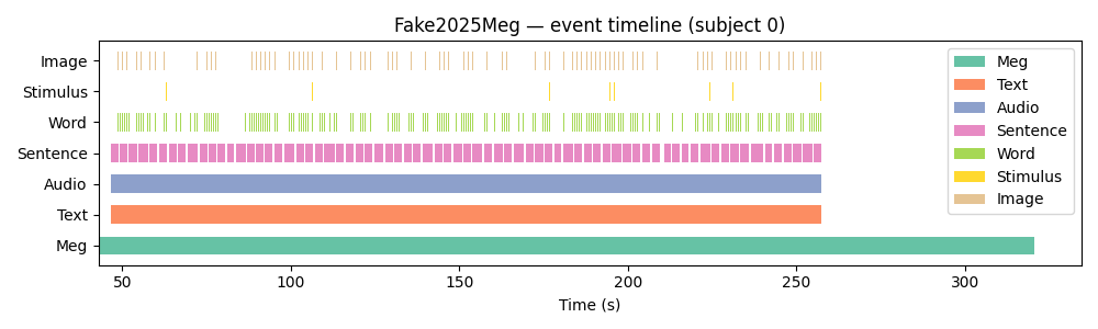
Visualise the timeline

import matplotlib.pyplot as plt

fig, ax = plt.subplots(figsize=(10, 3))
types = events["type"].unique()
colors = plt.cm.Set2(range(len(types)))

for i, t in enumerate(types):
    sub = events[events["type"] == t]
    ax.barh(
        i,
        sub["duration"].fillna(0.1),
        left=sub["start"],
        height=0.6,
        label=t,
        color=colors[i],
    )

ax.set_yticks(range(len(types)))
ax.set_yticklabels(types)
ax.set_xlabel("Time (s)")
ax.set_title("Fake2025Meg — event timeline (subject 0)")
ax.legend(loc="upper right")
plt.tight_layout()
plt.show()

Next: Create or share a study — wrap your own dataset as a Study subclass.