Adsorption Energies in MOFs

Pre-trained ODAC models are versatile across various MOF-related tasks. To begin, we’ll start with a fundamental application: calculating the adsorption energy for a single CO₂ molecule. This serves as an excellent and simple demonstration of what you can achieve with these datasets and models.

For predicting the adsorption energy of a single CO₂ molecule within a MOF structure, the adsorption energy ( $E_{\mathrm{ads}}$ ) is defined as:

E_{\mathrm{ads}} = E_{\mathrm{MOF+CO2}} - E_{\mathrm{MOF}} - E_{\mathrm{CO2}} \tag{1}

(1)

Each term on the right-hand side represents the energy of the relaxed state of the indicated chemical system. For a comprehensive understanding of our methodology for computing these adsorption energies, please refer to our paper.

Loading Pre-trained Models¶

Need to install fairchem-core or get UMA access or getting permissions/401 errors?

Install the necessary packages using pip, uv etc

! pip install fairchem-core fairchem-data-oc fairchem-applications-cattsunami

Get access to any necessary huggingface gated models
- Get and login to your Huggingface account
- Request access to https://huggingface.co/facebook/UMA
- Create a Huggingface token at https://huggingface.co/settings/tokens/ with the permission “Permissions: Read access to contents of all public gated repos you can access”
- Add the token as an environment variable using huggingface-cli login or by setting the HF_TOKEN environment variable.

# Login using the huggingface-cli utility
! huggingface-cli login

# alternatively,
import os
os.environ['HF_TOKEN'] = 'MY_TOKEN'

A pre-trained model can be loaded using FAIRChemCalculator. In this example, we’ll employ UMA to determine the CO₂ adsorption energies.

from fairchem.core import FAIRChemCalculator, pretrained_mlip

predictor = pretrained_mlip.get_predict_unit("uma-s-1p2")
calc = FAIRChemCalculator(predictor, task_name="odac")

WARNING:root:device was not explicitly set, using device='cuda'.

Adsorption in rigid MOFs: CO₂ Adsorption Energy in Mg-MOF-74¶

Let’s apply our knowledge to Mg-MOF-74, a widely studied MOF known for its excellent CO₂ adsorption properties. Its structure comprises magnesium atomic complexes connected by a carboxylated and oxidized benzene ring, serving as an organic linker. Previous studies consistently report the CO₂ adsorption energy for Mg-MOF-74 to be around -0.40 eV [1] [2] [3].

Our goal is to verify if we can achieve a similar value by performing a simple single-point calculation using UMA. In the ODAC23 dataset, all MOF structures are identified by their CSD (Cambridge Structural Database) code. For Mg-MOF-74, this code is OPAGIX. We’ve extracted a specific OPAGIX+CO2 configuration from the dataset, which exhibits the lowest adsorption energy among its counterparts.

import matplotlib.pyplot as plt
from ase.io import read
from ase.visualize.plot import plot_atoms

mof_co2 = read("structures/OPAGIX_w_CO2.cif")
mof = read("structures/OPAGIX.cif")
co2 = read("structures/co2.xyz")

fig, ax = plt.subplots(figsize=(5, 4.5), dpi=250)
plot_atoms(mof_co2, ax)
ax.set_axis_off()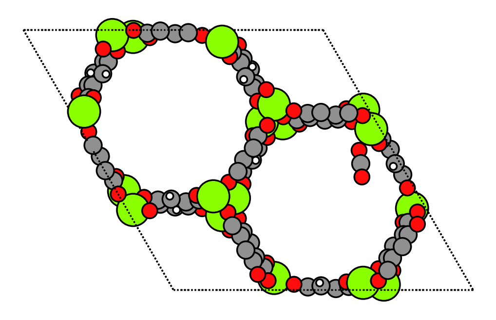

The final step in calculating the adsorption energy involves connecting the FAIRChemCalculator to each relaxed structure: OPAGIX+CO2, OPAGIX, and CO2. The structures used here are already relaxed from ODAC23. For simplicity, we assume here that further relaxations can be neglected. We will show how to go beyond this assumption in the next section.

mof_co2.calc = calc
mof.calc = calc
co2.calc = calc

E_ads = (
    mof_co2.get_potential_energy()
    - mof.get_potential_energy()
    - co2.get_potential_energy()
)

print(f"Adsorption energy of CO2 in Mg-MOF-74: {E_ads:.3f} eV")

WARNING:root:Model is being compiled this might take a while for the first time

W0916 12:47:44.128000 10329 site-packages/torch/_logging/_internal.py:1345] [0/0] Profiler record function <class 'torch.autograd.profiler.record_function'> will be ignored

WARNING:root:The UMA fast path (merge_mole + compile) is only available for fixed composition, task, charge, and spin. This is optimized for MD applications. Falling back to a less optimized version for subsequent evaluations. Reason: 'Compositions differ from merged model'.
Use inference_settings='batch' for heterogeneous batched evaluations.

Adsorption energy of CO2 in Mg-MOF-74: -0.473 eV

Adsorption in flexible MOFs¶

The adsorption energy calculation method outlined above is typically performed with rigid MOFs for simplicity. Both experimental and modeling literature have shown, however, that MOF flexibility can be important in accurately capturing the underlying chemistry of adsorption [1] [2] [3]. In particular, uptake can be improved by treating MOFs as flexible. Two types of MOF flexibility can be considered: intrinsic flexibility and deformation induced by guest molecules. In the Open DAC Project, we consider the latter MOF deformation by allowing the atomic positions of the MOF to relax during geometry optimization [4]. The addition of additional degrees of freedoms can complicate the computation of the adsorption energy and necessitates an extra step in the calculation procedure.

The figure below shows water adsorption in the MOF with CSD code WOBHEB with added defects (WOBHEB_0.11_0) from a DFT simulation. A typical adsorption energy calculation would only seek to capture the effects shaded in purple, which include both chemisorption and non-bonded interactions between the host and guest molecule. When allowing the MOF to relax, however, the adsorption energy also includes the energetic effect of the MOF deformation highlighted in green.

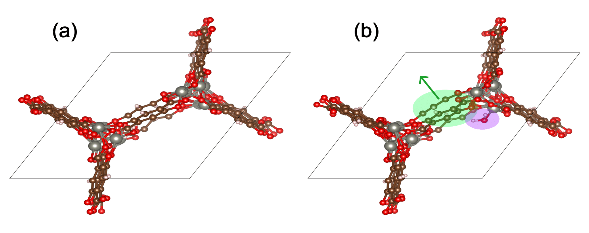
To account for this deformation, it is vital to use the most energetically favorable MOF geometry for the empty MOF term in Eqn. 1. Including MOF atomic coordinates as degrees of freedom can result in three possible outcomes:

The MOF does not deform, so the energies of the relaxed empty MOF and the MOF in the adsorbed state are the same
The MOF deforms to a less energetically favorable geometry than its ground state
The MOF locates a new energetically favorable geoemtry relative to the empty MOF relaxation

The first outcome requires no additional computation because the MOF rigidity assumption is valid. The second outcome represents physical and reversible deformation where the MOF returns to its empty ground state upon removal of the guest molecule. The third outcome is often the result of the guest molecule breaking local symmetry. We also found cases in ODAC in which both outcomes 2 and 3 occur within the same MOF.

To ensure the most energetically favorable empty MOF geometry is found, an addition empty MOF relaxation should be performed after MOF + adsorbate relaxation. The guest molecule should be removed, and the MOF should be relaxed starting from its geometry in the adsorbed state. If all deformation is reversible, the MOF will return to its original empty geometry. Otherwise, the lowest energy (most favorable) MOF geometry should be taken as the reference energy, $E_{\mathrm{MOF}}$ , in Eqn. 1.

H₂O Adsorption Energy in Flexible WOBHEB with UMA¶

The first part of this tutorial demonstrates how to perform a single point adsorption energy calculation using UMA. To treat MOFs as flexible, we perform all calculations on geometries determined by geometry optimization. The following example corresponds to the figure shown above (H₂O adsorption in WOBHEB_0.11_0).

In this tutorial, $E_{x}(r_{y})$ corresponds to the energy of $x$ determined from geometry optimization of $y$ .

First, we obtain the energy of the empty MOF from relaxation of only the MOF: $E_{\mathrm{MOF}}(r_{\mathrm{MOF}})$

import ase.io
from ase.optimize import BFGS

mof = ase.io.read("structures/WOBHEB_0.11.cif")
mof.calc = calc
relax = BFGS(mof)
relax.run(fmax=0.05)
E_mof_empty = mof.get_potential_energy()
print(f"Energy of empty MOF: {E_mof_empty:.3f} eV")

      Step     Time          Energy          fmax
BFGS:    0 12:48:41    -1077.368916        0.129115

BFGS:    1 12:48:44    -1077.370393        0.075187

BFGS:    2 12:48:48    -1077.372342        0.145326

BFGS:    3 12:48:49    -1077.374555        0.111782

BFGS:    4 12:48:53    -1077.376093        0.074286

BFGS:    5 12:48:57    -1077.377455        0.063782

BFGS:    6 12:48:59    -1077.378941        0.080853

BFGS:    7 12:48:59    -1077.380757        0.096832

BFGS:    8 12:49:02    -1077.382636        0.078391

BFGS:    9 12:49:03    -1077.384445        0.086898

BFGS:   10 12:49:06    -1077.386285        0.083308

BFGS:   11 12:49:09    -1077.388395        0.084005

BFGS:   12 12:49:11    -1077.390737        0.069075

BFGS:   13 12:49:12    -1077.393126        0.076051

BFGS:   14 12:49:13    -1077.395561        0.084263

BFGS:   15 12:49:15    -1077.398146        0.080029

BFGS:   16 12:49:15    -1077.400823        0.080008

BFGS:   17 12:49:16    -1077.403372        0.067395

BFGS:   18 12:49:16    -1077.405675        0.070430

BFGS:   19 12:49:19    -1077.407933        0.087880

BFGS:   20 12:49:19    -1077.410403        0.083992

BFGS:   21 12:49:20    -1077.413127        0.059536

BFGS:   22 12:49:21    -1077.415975        0.071944

BFGS:   23 12:49:24    -1077.418820        0.067787

BFGS:   24 12:49:24    -1077.421561        0.069914

BFGS:   25 12:49:26    -1077.424154        0.067345

BFGS:   26 12:49:27    -1077.426522        0.060821

BFGS:   27 12:49:27    -1077.428605        0.069356

BFGS:   28 12:49:28    -1077.430414        0.060308

BFGS:   29 12:49:28    -1077.432001        0.051483

BFGS:   30 12:49:28    -1077.433389        0.056298

BFGS:   31 12:49:29    -1077.434620        0.057605

BFGS:   32 12:49:30    -1077.435738        0.046080
Energy of empty MOF: -1077.436 eV

Next, we add the H₂O guest molecule and relax the MOF + adsorbate to obtain $E_{\mathrm{MOF+H2O}}(r_{\mathrm{MOF+H2O}})$ .

mof_h2o = ase.io.read("structures/WOBHEB_H2O.cif")
mof_h2o.calc = calc
relax = BFGS(mof_h2o)
relax.run(fmax=0.05)
E_combo = mof_h2o.get_potential_energy()
print(f"Energy of MOF + H2O: {E_combo:.3f} eV")

      Step     Time          Energy          fmax
BFGS:    0 12:49:31    -1091.661288        1.120236

BFGS:    1 12:49:31    -1091.679632        0.313939

BFGS:    2 12:49:32    -1091.683944        0.232090

BFGS:    3 12:49:33    -1091.695507        0.302352

BFGS:    4 12:49:35    -1091.701044        0.210409

BFGS:    5 12:49:35    -1091.707225        0.171332

BFGS:    6 12:49:36    -1091.712986        0.183112

BFGS:    7 12:49:36    -1091.720515        0.262525

BFGS:    8 12:49:37    -1091.727865        0.202908

BFGS:    9 12:49:37    -1091.735396        0.175156

BFGS:   10 12:49:38    -1091.743447        0.214444

BFGS:   11 12:49:38    -1091.752659        0.253378

BFGS:   12 12:49:42    -1091.762641        0.232723

BFGS:   13 12:49:45    -1091.773121        0.197381

BFGS:   14 12:49:48    -1091.784459        0.164070

BFGS:   15 12:49:52    -1091.796077        0.252814

BFGS:   16 12:49:53    -1091.806473        0.270217

BFGS:   17 12:49:54    -1091.815242        0.186113

BFGS:   18 12:49:54    -1091.822968        0.130980

BFGS:   19 12:49:55    -1091.830281        0.120378

BFGS:   20 12:49:57    -1091.837495        0.140834

BFGS:   21 12:49:58    -1091.844733        0.154664

BFGS:   22 12:49:58    -1091.851967        0.162360

BFGS:   23 12:49:59    -1091.858819        0.164805

BFGS:   24 12:50:02    -1091.864230        0.167649

BFGS:   25 12:50:06    -1091.868702        0.416135

BFGS:   26 12:50:08    -1091.873929        0.220544

BFGS:   27 12:50:11    -1091.880101        0.092246

BFGS:   28 12:50:14    -1091.884366        0.090918

BFGS:   29 12:50:14    -1091.889008        0.138150

BFGS:   30 12:50:15    -1091.893530        0.143174

BFGS:   31 12:50:15    -1091.899478        0.224470

BFGS:   32 12:50:19    -1091.904702        0.300773

BFGS:   33 12:50:20    -1091.908756        0.353395

BFGS:   34 12:50:22    -1091.913993        0.193329

BFGS:   35 12:50:23    -1091.920799        0.150868

BFGS:   36 12:50:25    -1091.927043        0.161484

BFGS:   37 12:50:26    -1091.934428        0.329386

BFGS:   38 12:50:26    -1091.939555        0.150915

BFGS:   39 12:50:27    -1091.944250        0.554904

BFGS:   40 12:50:27    -1091.951894        0.210117

BFGS:   41 12:50:29    -1091.959240        0.162422

BFGS:   42 12:50:31    -1091.969225        0.255163

BFGS:   43 12:50:33    -1091.978703        0.203654

BFGS:   44 12:50:36    -1091.987553        0.643538

BFGS:   45 12:50:36    -1091.996516        0.460747

BFGS:   46 12:50:37    -1092.010956        0.252388

BFGS:   47 12:50:38    -1092.028185        0.384759

BFGS:   48 12:50:41    -1092.043254        0.819555

BFGS:   49 12:50:44    -1092.066557        0.418108

BFGS:   50 12:50:44    -1092.093803        0.341144

BFGS:   51 12:50:45    -1092.110960        0.719880

BFGS:   52 12:50:45    -1092.120459        0.468311

BFGS:   53 12:50:46    -1092.145171        0.347964

BFGS:   54 12:50:46    -1092.160172        0.447638

BFGS:   55 12:50:48    -1092.174393        0.344564

BFGS:   56 12:50:49    -1092.190632        0.303262

BFGS:   57 12:50:50    -1092.209693        0.325326

BFGS:   58 12:50:51    -1092.219857        0.317897

BFGS:   59 12:50:53    -1092.233834        0.333360

BFGS:   60 12:50:54    -1092.246443        0.288916

BFGS:   61 12:50:57    -1092.257707        0.253072

BFGS:   62 12:51:00    -1092.265241        0.183778

BFGS:   63 12:51:01    -1092.271661        0.149763

BFGS:   64 12:51:05    -1092.277848        0.119049

BFGS:   65 12:51:05    -1092.283553        0.110318

BFGS:   66 12:51:07    -1092.288491        0.143468

BFGS:   67 12:51:08    -1092.293166        0.165306

BFGS:   68 12:51:11    -1092.297849        0.122420

BFGS:   69 12:51:12    -1092.302214        0.100999

BFGS:   70 12:51:12    -1092.306156        0.128527

BFGS:   71 12:51:13    -1092.310193        0.136490

BFGS:   72 12:51:16    -1092.314604        0.147574

BFGS:   73 12:51:18    -1092.319059        0.131982

BFGS:   74 12:51:21    -1092.323015        0.117578

BFGS:   75 12:51:24    -1092.326454        0.087855

BFGS:   76 12:51:26    -1092.329640        0.116636

BFGS:   77 12:51:26    -1092.332517        0.095784

BFGS:   78 12:51:30    -1092.334803        0.055318

BFGS:   79 12:51:34    -1092.336503        0.057614

BFGS:   80 12:51:34    -1092.337874        0.055937

BFGS:   81 12:51:39    -1092.339167        0.065012

BFGS:   82 12:51:39    -1092.340514        0.057358

BFGS:   83 12:51:41    -1092.341917        0.065093

BFGS:   84 12:51:44    -1092.343318        0.067003

BFGS:   85 12:51:45    -1092.344694        0.079053

BFGS:   86 12:51:46    -1092.346037        0.065644

BFGS:   87 12:51:46    -1092.347346        0.052881

BFGS:   88 12:51:46    -1092.348559        0.046092
Energy of MOF + H2O: -1092.349 eV

We can now isolate the MOF atoms from the relaxed MOF + H₂O geometry and see that the MOF has adopted a geometry that is less energetically favorable than the empty MOF by ~0.2 eV. The energy of the MOF in the adsorbed state corresponds to $E_{\mathrm{MOF}}(r_{\mathrm{MOF+H2O}})$ .

mof_adsorbed_state = mof_h2o[:-3]
mof_adsorbed_state.calc = calc
E_mof_adsorbed_state = mof_adsorbed_state.get_potential_energy()
print(f"Energy of MOF in the adsorbed state: {E_mof_adsorbed_state:.3f} eV")

Energy of MOF in the adsorbed state: -1077.150 eV

H₂O adsorption in this MOF appears to correspond to Case #2 as outlined above. We can now perform re-relaxation of the empty MOF starting from the $r_{\mathrm{MOF+H2O}}$ geometry.

relax = BFGS(mof_adsorbed_state)
relax.run(fmax=0.05)
E_mof_rerelax = mof_adsorbed_state.get_potential_energy()
print(f"Energy of re-relaxed empty MOF: {E_mof_rerelax:.3f} eV")

      Step     Time          Energy          fmax
BFGS:    0 12:51:47    -1077.149955        1.015144

BFGS:    1 12:51:47    -1077.191027        0.890129

BFGS:    2 12:51:50    -1077.242119        0.657896

BFGS:    3 12:51:54    -1077.289397        0.488875

BFGS:    4 12:51:58    -1077.307194        0.358901

BFGS:    5 12:51:59    -1077.323867        0.298828

BFGS:    6 12:51:59    -1077.337783        0.322128

BFGS:    7 12:52:02    -1077.350158        0.257647

BFGS:    8 12:52:02    -1077.357388        0.134678

BFGS:    9 12:52:03    -1077.362213        0.127175

BFGS:   10 12:52:03    -1077.366732        0.178157

BFGS:   11 12:52:03    -1077.371423        0.173272

BFGS:   12 12:52:04    -1077.376203        0.139286

BFGS:   13 12:52:05    -1077.380922        0.125096

BFGS:   14 12:52:06    -1077.385506        0.150033

BFGS:   15 12:52:09    -1077.389464        0.127395

BFGS:   16 12:52:10    -1077.392548        0.090776

BFGS:   17 12:52:11    -1077.395227        0.092744

BFGS:   18 12:52:13    -1077.397931        0.115422

BFGS:   19 12:52:14    -1077.400646        0.114132

BFGS:   20 12:52:17    -1077.403323        0.103942

BFGS:   21 12:52:21    -1077.405949        0.099276

BFGS:   22 12:52:23    -1077.408488        0.084677

BFGS:   23 12:52:27    -1077.410848        0.095028

BFGS:   24 12:52:28    -1077.412961        0.075087

BFGS:   25 12:52:28    -1077.414857        0.076629

BFGS:   26 12:52:32    -1077.416565        0.078824

BFGS:   27 12:52:36    -1077.418017        0.079751

BFGS:   28 12:52:39    -1077.419245        0.049366
Energy of re-relaxed empty MOF: -1077.419 eV

The MOF returns to its original empty reference energy upon re-relaxation, confirming that this deformation is physically relevant and is induced by the adsorbate molecule. In Case #3, this re-relaxed energy will be more negative (more favorable) than the original empty MOF relaxation. Thus, we take the reference empty MOF energy ( $E_{\mathrm{MOF}}$ in Eqn. 1) to be the minimum of the original empty MOF energy and the re-relaxed MOf energy:

E_mof = min(E_mof_empty, E_mof_rerelax)

# get adsorbate reference energy
h2o = mof_h2o[-3:]
h2o.calc = calc
E_h2o = h2o.get_potential_energy()

# compute adsorption energy
E_ads = E_combo - E_mof - E_h2o
print(f"Adsorption energy of H2O in WOBHEB_0.11_0: {E_ads:.3f} eV")

Adsorption energy of H2O in WOBHEB_0.11_0: -0.539 eV

This adsorption energy closely matches that from DFT (–0.699 eV) [1]. The strong adsorption energy is a consequence of both H₂O chemisorption and MOF deformation. We can decompose the adsorption energy into contributions from these two factors. Assuming rigid H₂O molecules, we define $E_{\mathrm{int}}$ and $E_{\mathrm{MOF,deform}}$ , respectively, as

E_{\mathrm{int}} = E_{\mathrm{MOF+H2O}}(r_{\mathrm{MOF+H2O}}) - E_{\mathrm{MOF}}(r_{\mathrm{MOF+H2O}}) - E_{\mathrm{H2O}}(r_{\mathrm{MOF+H2O}}) \tag{2}

(2)

E_{\mathrm{MOF,deform}} = E_{\mathrm{MOF}}(r_{\mathrm{MOF+H2O}}) - E_{\mathrm{MOF}}(r_{\mathrm{MOF}}) \tag{3}

(3)

$E_{\mathrm{int}}$ describes host host–guest interactions for the MOF in the adsorbed state only. $E_{\mathrm{MOF,deform}}$ quantifies the magnitude of deformation between the MOF in the adsorbed state and the most energetically favorable empty MOF geometry determined from the workflow presented here. It can be shown that

E_{\mathrm{ads}} = E_{\mathrm{int}} + E_{\mathrm{MOF,deform}} \tag{4}

(4)

For H₂O adsorption in WOBHEB_0.11, we have

E_int = E_combo - E_mof_adsorbed_state - E_h2o
print(f"E_int: {E_int}")

E_int: -0.8247172034400005

E_mof_deform = E_mof_adsorbed_state - E_mof_empty
print(f"E_mof_deform: {E_mof_deform}")

E_mof_deform: 0.28578329426841265

E_ads = E_int + E_mof_deform
print(f"E_ads: {E_ads}")

E_ads: -0.5389339091715879

$E_{\mathrm{int}}$ is equivalent to $E_{\mathrm{ads}}$ when the MOF is assumed to be rigid. In this case, failure to consider adsorbate-induced deformation would result in an overestimation of the adsorption energy magnitude.

Acknowledgements & Authors¶

Logan Brabson and Sihoon Choi (Georgia Tech) and the OpenDAC project.

References¶

Sriram, A., Choi, S., Yu, X., Brabson, L. M., Das, A., Ulissi, Z., Uyttendaele, M., Medford, A. J., & Sholl, D. S. (2024). The Open DAC 2023 Dataset and Challenges for Sorbent Discovery in Direct Air Capture. ACS Central Science, 10(5), 923–941. 10.1021/acscentsci.3c01629
Queen, W. L., Hudson, M. R., Bloch, E. D., Mason, J. A., Gonzalez, M. I., Lee, J. S., Gygi, D., Howe, J. D., Lee, K., Darwish, T. A., James, M., Peterson, V. K., Teat, S. J., Smit, B., Neaton, J. B., Long, J. R., & Brown, C. M. (2014). Comprehensive study of carbon dioxide adsorption in the metal–organic frameworks M 2 (dobdc) (M = Mg, Mn, Fe, Co, Ni, Cu, Zn). Chem. Sci., 5(12), 4569–4581. 10.1039/c4sc02064b
Yu, D., Yazaydin, A. O., Lane, J. R., Dietzel, P. D. C., & Snurr, R. Q. (2013). A combined experimental and quantum chemical study of CO2 adsorption in the metal–organic framework CPO-27 with different metals. Chemical Science, 4(9), 3544. 10.1039/c3sc51319j
Alonso, G., Bahamon, D., Keshavarz, F., Giménez, X., Gamallo, P., & Sayós, R. (2018). Density Functional Theory-Based Adsorption Isotherms for Pure and Flue Gas Mixtures on Mg-MOF-74. Application in CO2 Capture Swing Adsorption Processes. The Journal of Physical Chemistry C, 122(7), 3945–3957. 10.1021/acs.jpcc.8b00938
Witman, M., Ling, S., Jawahery, S., Boyd, P. G., Haranczyk, M., Slater, B., & Smit, B. (2017). The Influence of Intrinsic Framework Flexibility on Adsorption in Nanoporous Materials. Journal of the American Chemical Society, 139(15), 5547–5557. 10.1021/jacs.7b01688

Loading Pre-trained Models¶

Adsorption in rigid MOFs: CO2 Adsorption Energy in Mg-MOF-74¶

Adsorption in flexible MOFs¶

H2O Adsorption Energy in Flexible WOBHEB with UMA¶

Acknowledgements & Authors¶

Adsorption in rigid MOFs: CO₂ Adsorption Energy in Mg-MOF-74¶

H₂O Adsorption Energy in Flexible WOBHEB with UMA¶